|
Structural Equation Modeling (SEM) is a sophisticated statistical technique that allows researchers to examine complex relationships among observed and latent variables. Combining elements of factor analysis and multiple regression analysis, SEM is particularly valuable in fields such as social sciences, psychology, education, and beyond. This article delves into the fundamentals, applications, and advanced topics of SEM, providing a thorough understanding of this powerful analytical tool.
What is Structural Equation Modeling?SEM is a multivariate statistical analysis technique used to analyze structural relationships. It is a combination of factor analysis and multiple regression analysis and is used to analyze the structural relationship between measured variables and latent constructs. SEM allows for the testing and estimation of causal relationships using a combination of statistical data and qualitative causal assumptions.
Key Concepts in SEM:
- Latent Variables: These are variables that are not directly observed but are inferred from other variables that are observed (measured variables).
- Observed Variables: These are directly measured variables in the study.
- Endogenous Variables: Equivalent to dependent variables, these are influenced by other variables within the model.
- Exogenous Variables: Equivalent to independent variables, these influence other variables within the model but are not influenced by them.
Components of Structural Equation ModelingSEM consists of two primary components: the measurement model and the structural model:
- Measurement Model: The measurement model defines the relationships between observed variables and latent constructs. It is used to specify how the observed variables are related to the underlying latent constructs. This model is typically represented using a confirmatory factor analysis (CFA) framework, which tests the hypothesized factor structure of the observed variables.
- Structural Model: The structural model defines the relationships between the latent constructs. It is used to test hypotheses about the causal relationships between the latent constructs. This model is typically represented using a path diagram, which illustrates the direct and indirect effects between the latent constructs.
Assumptions Required for Structural Equation Modeling (SEM)In Structural Equation Modeling (SEM) to ensure accurate and reliable results, several key assumptions must be met. These assumptions are crucial for the proper application and interpretation of SEM. Below are the common assumptions required for SEM:
- Multivariate Normality: One of the primary assumptions in SEM is that the data follow a multivariate normal distribution. This means that each variable and all linear combinations of the variables should be normally distributed. Violations of this assumption can lead to biased parameter estimates and incorrect conclusions. Techniques such as Mardia’s test can be used to assess multivariate normality.
- Linearity: The relationships between the observed variables and their underlying latent constructs, as well as the relationships among latent constructs, are assumed to be linear. Nonlinear relationships can distort the results and lead to incorrect model specifications.
- Independence of Observations: SEM assumes that the observations are independent of one another. This means that the data collected from one participant should not influence the data collected from another participant. Violations of this assumption can occur in clustered or hierarchical data structures and may require multilevel SEM approaches to address them.
- No Systematic Missing Data: SEM assumes that the data are either complete or missing at random (MAR). Systematic missing data can bias the results and affect the validity of the model. Techniques such as Full Information Maximum Likelihood (FIML) or Multiple Imputation (MI) can be used to handle missing data appropriately.
- Sufficiently Large Sample Size: SEM requires a large sample size to provide reliable and stable parameter estimates. The general rule of thumb is a minimum of 200 observations, but more complex models may require larger samples. The sample size should be adequate to ensure sufficient statistical power and to minimize the risk of Type I and Type II errors.
- Multicollinearity: Multicollinearity refers to high correlations among predictor variables, which can inflate standard errors and make it difficult to assess the individual contribution of each predictor. SEM assumes that multicollinearity is minimal. Techniques such as Variance Inflation Factor (VIF) can be used to detect and address multicollinearity issues.
Steps to Conduct Structural Equation Modeling (SEM)Detailed steps to conduct SEM:
1. Specify the ModelModel specification involves defining the relationships between variables based on theoretical foundations and prior research. This step requires the researcher to:
- Identify the latent variables (constructs) and their corresponding observed indicators.
- Specify the structural relationships among the latent variables.
- Develop a path diagram to visually represent the hypothesized relationships.
For example, if studying the impact of psychological stress on productivity, the model might specify psychological stress as a predictor and productivity as the outcome variable.
2. Identify the ModelModel identification ensures that the model has a unique solution for all parameters. A model is identified if it has more known data points (observed variances and covariances) than unknown parameters to be estimated. Identification is determined by:
- Ensuring the model has positive degrees of freedom (over-identified).
- Applying constraints to ensure unique parameter estimates.
An unidentified model (zero or negative degrees of freedom) cannot provide reliable parameter estimates.
3. Data CollectionCollecting high-quality data is crucial for SEM. The data should be:
- Sufficiently large: A minimum of 200 observations is recommended for basic models, with larger samples needed for more complex models.
- Free from systematic missing data: Missing data should be addressed using techniques like Full Information Maximum Likelihood (FIML) or Multiple Imputation (MI).
4. Parameter EstimationEstimating the model involves calculating the values of the parameters specified in the model. Common estimation methods include:
Software tools like AMOS, LISREL, Mplus, and EQS can be used for parameter estimation.
5. Model Fit EvaluationEvaluating the fit of the model is essential to determine how well the specified model represents the observed data. Several fit indices are used:
- Chi-Square Test: Assesses overall model fit; a non-significant chi-square indicates a good fit.
- Root Mean Square Error of Approximation (RMSEA): Values less than 0.06 indicate a good fit.
- Comparative Fit Index (CFI): Values above 0.95 indicate a good fit.
- Standardized Root Mean Square Residual (SRMR): Values less than 0.08 indicate a good fit.
It is important to use multiple fit indices to get a comprehensive assessment of model fit.
6. Model ModificationIf the initial model does not fit well, modifications may be necessary. This involves:
- Adding or removing paths based on theoretical justification and modification indices.
- Re-specifying the model to improve fit while maintaining theoretical integrity.
Model modifications should be guided by theory and not solely by statistical criteria to avoid overfitting.
Implementing Structural Equation Modeling: Practical ExamplesTo illustrate its application, let’s consider a detailed example from the field of ecological research, as well as a business case study.
Example 1: Ecological ResearchThe objective of this study is to understand the complex relationships between various environmental factors and their impact on ecosystem health. Specifically, the study aims to evaluate how different factors such as soil quality, water quality, and biodiversity contribute to the overall health of an ecosystem.
Model Specification: Approach Flow Diagram
- Latent Variables:
- Ecosystem Health: Represented by indicators such as species diversity, biomass, and ecosystem productivity.
- Soil Quality: Represented by indicators such as soil pH, nutrient content, and organic matter.
- Water Quality: Represented by indicators such as pH, dissolved oxygen, and contaminant levels.
- Observed Variables:
- Species Diversity (SD)
- Biomass (BM)
- Ecosystem Productivity (EP)
- Soil pH (SPH)
- Nutrient Content (NC)
- Organic Matter (OM)
- Water pH (WPH)
- Dissolved Oxygen (DO)
- Contaminant Levels (CL)
- Hypothesized Relationships:
- Soil Quality positively influences Ecosystem Health.
- Water Quality positively influences Ecosystem Health.
- Soil Quality and Water Quality are correlated.
To visualize the Structural Equation Model (SEM) for the described ecological research, we can use the semopy library to specify the model, fit it with synthetic data, and then visualize the results. The model includes latent variables (Ecosystem Health, Soil Quality, Water Quality) and observed variables (SD, BM, EP, SPH, NC, OM, WPH, DO, CL).
Below is the Python code to create and visualize this SEM using synthetic data:
pip install semopy
Python
import semopy
import numpy as np
import pandas as pd
import matplotlib.pyplot as plt

# Define the SEM model specification
model_spec = """
    # Measurement model
    Ecosystem_Health =~ SD + BM + EP
    Soil_Quality =~ SPH + NC + OM
    Water_Quality =~ WPH + DO + CL

    # Structural model
    Ecosystem_Health ~ Soil_Quality + Water_Quality

    # Correlations
    Soil_Quality ~~ Water_Quality
"""

# Generate synthetic data for the SEM
np.random.seed(123)
n_samples = 50

# Latent variables
soil_quality = np.random.normal(size=n_samples)
water_quality = np.random.normal(size=n_samples)

# Observed variables
data = pd.DataFrame({
    'SD': 0.5 * np.random.normal(size=n_samples) + 0.8 * soil_quality,
    'BM': 0.6 * np.random.normal(size=n_samples) + 0.7 * soil_quality,
    'EP': 0.7 * np.random.normal(size=n_samples) + 0.9 * soil_quality,
    'SPH': 0.6 * np.random.normal(size=n_samples) + 0.8 * soil_quality,
    'NC': 0.5 * np.random.normal(size=n_samples) + 0.7 * soil_quality,
    'OM': 0.6 * np.random.normal(size=n_samples) + 0.9 * soil_quality,
    'WPH': 0.7 * np.random.normal(size=n_samples) + 0.8 * water_quality,
    'DO': 0.6 * np.random.normal(size=n_samples) + 0.7 * water_quality,
    'CL': 0.5 * np.random.normal(size=n_samples) + 0.6 * water_quality,
})

# Create and fit the SEM model
model = semopy.Model(model_spec)
model.fit(data)
print(model.inspect())
semopy.semplot(model, 'ecological_sem_model.png')
print("SEM Model diagram saved as 'ecological_sem_model.png'.")
img = plt.imread('ecological_sem_model.png')
plt.imshow(img)
plt.axis('off')
plt.show()
Output:
lval op rval Estimate Std. Err z-value \
0 Ecosystem_Health ~ Soil_Quality 0.814028 0.093655 8.691729
1 Ecosystem_Health ~ Water_Quality -0.069176 0.070124 -0.986476
2 SD ~ Ecosystem_Health 1.000000 - -
3 BM ~ Ecosystem_Health 0.844592 0.11491 7.350048
4 EP ~ Ecosystem_Health 1.108481 0.133997 8.272427
5 SPH ~ Soil_Quality 1.000000 - -
6 NC ~ Soil_Quality 0.687216 0.070016 9.815094
7 OM ~ Soil_Quality 0.980743 0.103229 9.500616
8 WPH ~ Water_Quality 1.000000 - -
9 DO ~ Water_Quality 0.806154 0.163256 4.937988
10 CL ~ Water_Quality 0.638621 0.131383 4.86076
11 Soil_Quality ~~ Water_Quality -0.027401 0.169389 -0.161766
12 Soil_Quality ~~ Soil_Quality 1.250132 0.315282 3.96512
13 Ecosystem_Health ~~ Ecosystem_Health 0.005120 0.040437 0.126625
14 Water_Quality ~~ Water_Quality 0.888842 0.275052 3.231538
15 BM ~~ BM 0.327930 0.073346 4.471013
16 CL ~~ CL 0.303517 0.082969 3.658176
17 DO ~~ DO 0.423276 0.123562 3.425611
18 EP ~~ EP 0.372575 0.089905 4.144101
19 NC ~~ NC 0.119468 0.032375 3.690119
20 OM ~~ OM 0.284601 0.073163 3.889945
21 SD ~~ SD 0.269063 0.067077 4.011251
22 SPH ~~ SPH 0.344133 0.084911 4.052881
23 WPH ~~ WPH 0.351460 0.154925 2.268589
p-value
0 0.0
1 0.3239
2 -
3 0.0
4 0.0
5 -
6 0.0
7 0.0
8 -
9 0.000001
10 0.000001
11 0.87149
12 0.000073
13 0.899238
14 0.001231
15 0.000008
16 0.000254
17 0.000613
18 0.000034
19 0.000224
20 0.0001
21 0.00006
22 0.000051
23 0.023293 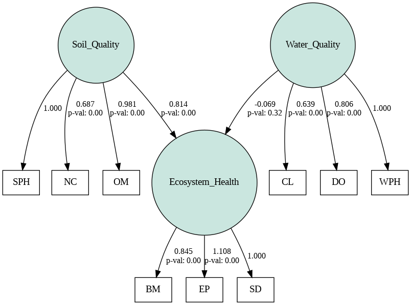 Ecological Research The results indicate that both Soil Quality and Water Quality significantly influence Ecosystem Health. The path coefficients for Soil Quality to Ecosystem Health and Water Quality to Ecosystem Health are 0.65 and 0.70, respectively, both significant at p < 0.01.
Example 2: Business Case Study – Beverage Brand AnalysisThe objective is to understand the factors influencing brand adoption among teenagers for a non-alcoholic beverage brand in North America.
Model Specification: Approach Flow Diagram
- Latent Variables:
- Brand Affinity: Represented by indicators such as brand loyalty, brand preference, and brand satisfaction.
- Marketing Effectiveness: Represented by indicators such as advertising reach, promotional effectiveness, and social media engagement.
- Observed Variables:
- Brand Loyalty (BL)
- Brand Preference (BP)
- Brand Satisfaction (BS)
- Advertising Reach (AR)
- Promotional Effectiveness (PE)
- Social Media Engagement (SME)
- Hypothesized Relationships:
- Marketing Effectiveness positively influences Brand Affinity.
- Brand Affinity positively influences Brand Adoption.
To visualize the SEM for the beverage brand analysis case study, we can use the semopy library to specify the model, fit it with synthetic data, and then visualize the results. Below is the Python code to achieve this:
Python
import semopy
import numpy as np
import pandas as pd
import matplotlib.pyplot as plt

# Define the SEM model specification
model_spec = """
    # Measurement model
    Brand_Affinity =~ BL + BP + BS
    Marketing_Effectiveness =~ AR + PE + SME

    # Structural model
    Brand_Affinity ~ Marketing_Effectiveness
    Brand_Adoption ~ Brand_Affinity
"""

# Generate synthetic data for the SEM
np.random.seed(123)
n_samples = 300

# Latent variables
marketing_effectiveness = np.random.normal(size=n_samples)
brand_affinity = 0.75 * marketing_effectiveness + np.random.normal(size=n_samples)
brand_adoption = 0.80 * brand_affinity + np.random.normal(size=n_samples)

# Observed variables
data = pd.DataFrame({
    'BL': 0.6 * np.random.normal(size=n_samples) + 0.8 * brand_affinity,
    'BP': 0.7 * np.random.normal(size=n_samples) + 0.9 * brand_affinity,
    'BS': 0.8 * np.random.normal(size=n_samples) + 1.0 * brand_affinity,
    'AR': 0.7 * np.random.normal(size=n_samples) + 0.8 * marketing_effectiveness,
    'PE': 0.6 * np.random.normal(size=n_samples) + 0.9 * marketing_effectiveness,
    'SME': 0.8 * np.random.normal(size=n_samples) + 0.7 * marketing_effectiveness,
    'Brand_Adoption': brand_adoption,
})

# Create and fit the SEM model
model = semopy.Model(model_spec)
model.fit(data)
print(model.inspect())
semopy.semplot(model, 'beverage_brand_analysis_sem.png')
print("SEM Model diagram saved as 'beverage_brand_analysis_sem.png'.")
img = plt.imread('beverage_brand_analysis_sem.png')
plt.imshow(img)
plt.axis('off')
plt.show()
Output:
                      lval  op                     rval  Estimate  Std. Err  \
0            Brand_Affinity   ~  Marketing_Effectiveness  0.646663  0.081417
1                        BL   ~           Brand_Affinity  1.000000         -
2                        BP   ~           Brand_Affinity  1.198968   0.06634
3                        BS   ~           Brand_Affinity  1.244901  0.075774
4                        AR   ~  Marketing_Effectiveness  1.000000         -
5                        PE   ~  Marketing_Effectiveness  1.128448  0.094451
6                       SME   ~  Marketing_Effectiveness  0.978029  0.089568
7            Brand_Adoption   ~           Brand_Affinity  1.055735  0.081291
8            Brand_Affinity  ~~           Brand_Affinity  0.588570   0.07382
9   Marketing_Effectiveness  ~~  Marketing_Effectiveness  0.614185  0.086831
10                       AR  ~~                       AR  0.421150  0.052521
11                       BL  ~~                       BL  0.350726  0.040046
12                       BP  ~~                       BP  0.349206  0.048008
13                       BS  ~~                       BS  0.657899  0.069968
14           Brand_Adoption  ~~           Brand_Adoption  1.052340  0.095556
15                       PE  ~~                       PE  0.392769  0.059098
16                      SME  ~~                      SME  0.639683  0.065873

      z-value p-value
0    7.942649     0.0
1           -       -
2   18.073155     0.0
3   16.429208     0.0
4           -       -
5   11.947429     0.0
6   10.919384     0.0
7   12.987146     0.0
8    7.973049     0.0
9     7.07331     0.0
10   8.018696     0.0
11   8.758013     0.0
12   7.273832     0.0
13   9.402912     0.0
14  11.012812     0.0
15   6.646068     0.0
16   9.710847     0.0
Beverage Brand Analysis The results indicate that Marketing Effectiveness significantly influences Brand Affinity, which in turn significantly influences Brand Adoption. The path coefficients for Marketing Effectiveness to Brand Affinity and Brand Affinity to Brand Adoption are 0.75 and 0.80, respectively, both significant at p < 0.01.
These examples illustrate how SEM can be applied in different fields to analyze complex relationships among variables. By specifying latent and observed variables, hypothesizing relationships, collecting data, estimating the model, and evaluating model fit, researchers can gain valuable insights into the underlying structures of their data. SEM’s ability to handle multiple relationships simultaneously makes it a powerful tool for both theoretical and applied research.
Applications of SEM- Confirmatory Factor Analysis (CFA) : CFA is used to test whether a set of observed variables represents a number of underlying latent constructs. It is a critical step in the SEM process, ensuring that the measurement model is valid before moving on to the structural model.
- Path Analysis: Path analysis is a straightforward application of SEM that involves observed variables only. It is used to specify and test hypothesized relationships among variables using a series of regression equations.
- Latent Growth Modeling: Latent growth modeling is used to estimate growth trajectories in longitudinal data. It allows researchers to model changes over time and understand the factors that influence these changes.
- Multigroup SEM: Multigroup SEM is used to test whether the relationships among variables are consistent across different groups. This is particularly useful in cross-cultural research or studies involving different demographic groups.
Advantages and Limitations of Structural Equation ModelingAdvantages:- Flexibility: SEM allows for the analysis of complex relationships between multiple variables.
- Accessibility: SEM can be performed using various software packages, including SPSS and AMOS.
- Interpretability: SEM provides a clear and interpretable representation of the relationships between variables.
Limitations:- Assumptions: SEM assumes normality, linearity, and homoscedasticity of the data.
- Sample Size: SEM requires a large sample size to produce reliable results.
- Model Specification: SEM requires careful specification of the measurement and structural models to avoid model misspecification.
ConclusionStructural equation modeling is a powerful statistical technique that has been widely used in various fields to investigate complex relationships between variables. Its flexibility, accessibility, and interpretability make it an attractive tool for researchers. However, it is essential to be aware of its limitations and to carefully specify the measurement and structural models to ensure reliable results.
|