Logistic regression is a powerful statistical method used for modeling binary outcomes. When applying logistic regression in practice, one common challenge is deciding the threshold probability that determines the classification of observations into binary classes (e.g., yes/no, 1/0). This article explores various approaches and considerations for determining an appropriate threshold for a generalized linear model (GLM) in R.

Importance of Threshold Selection

After fitting a logistic regression model, predictions are based on the predicted probabilities. These probabilities can then be converted into class predictions (e.g., 0 or 1) using a threshold. The choice of threshold directly impacts the model’s classification performance, including metrics such as accuracy, sensitivity, specificity, and the ROC curve.

Methods for Deciding Threshold

Here we discuss the main Methods for Deciding Thresholds in the R Programming Language.

• Default Threshold (0.5): The default threshold commonly used is 0.5, where predictions above 0.5 are classified as one class, and below 0.5 as the other. This threshold is intuitive but may not always be optimal depending on the specific application.
• ROC Curve Analysis: Receiver Operating Characteristic (ROC) curves plot the true positive rate (sensitivity) against the false positive rate (1-specificity) for different threshold values. The Area Under the Curve (AUC) summarizes the ROC curve’s performance across all possible thresholds. Optimal thresholds often maximize sensitivity and specificity or are selected based on domain-specific considerations.
• Precision-Recall Curve Analysis: Precision-Recall (PR) curves plot precision (positive predictive value) against recall (sensitivity) for different thresholds. They are particularly useful when dealing with imbalanced datasets where one class is much rarer than the other.
• Cost-Sensitive Analysis: In some applications, misclassifying one class (e.g., false positives or false negatives) may have different costs or implications. Decision theory and cost-sensitive analysis help determine thresholds that minimize expected costs or maximize utility.
• Domain Knowledge and Context: Understanding the domain-specific implications of misclassifications is crucial. The threshold should align with the practical consequences of classification errors in the specific application.

Step 1: Load Required Libraries and Dataset

We’ll use the pROC package for ROC curve analysis and the caret package for data preprocessing. For this example, let’s consider the famous Pima Indians Diabetes Database from the caret package, which contains information about diabetic and non-diabetic patients.

# Install and load necessary packages
install.packages("pROC")
install.packages("caret")

library(pROC)
library(caret)

# Load necessary dataset
data(PimaIndiansDiabetes, package = "mlbench")

# Inspect the first few rows of the dataset
head(PimaIndiansDiabetes)

Output:

  pregnant glucose pressure triceps insulin mass pedigree age diabetes
1        6     148       72      35       0 33.6    0.627  50      pos
2        1      85       66      29       0 26.6    0.351  31      neg
3        8     183       64       0       0 23.3    0.672  32      pos
4        1      89       66      23      94 28.1    0.167  21      neg
5        0     137       40      35     168 43.1    2.288  33      pos
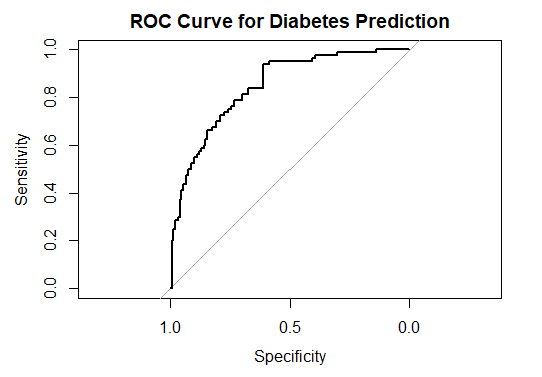
6        5     116       74       0       0 25.6    0.201  30      neg

Step 2: Preprocess and Split Data

Now we will Preprocess and Split Data into training and testing.

# Data preprocessing
set.seed(123)  # Set seed for reproducibility
trainIndex <- createDataPartition(PimaIndiansDiabetes$diabetes, p = 0.7, list = FALSE)
data_train <- PimaIndiansDiabetes[trainIndex, ]
data_test <- PimaIndiansDiabetes[-trainIndex, ]

Step 3: Fit Logistic Regression Model

Now we will fit Logistic Regression Model.

# Fit logistic regression model
model <- glm(diabetes ~ ., data = data_train, family = "binomial")

# Predict probabilities on test data
predicted_prob <- predict(model, newdata = data_test, type = "response")

Step 4: ROC Curve Analysis

Now we will perform ROC Curve Analysis.

# Create ROC curve
roc_curve <- roc(data_test$diabetes, predicted_prob)

# Plot ROC curve
plot(roc_curve, main = "ROC Curve for Diabetes Prediction")

Output:

Deciding threshold for glm logistic regression model in R

Step 5: Determine Optimal Threshold

At last we will Determine Optimal Threshold.

# Identify threshold maximizing sensitivity and specificity
coords <- coords(roc_curve, "best", best.method = "closest.topleft")
best_threshold <- coords$threshold

cat("Optimal threshold based on ROC curve:", best_threshold, "\n")

# Predict classes based on optimal threshold
predicted_class <- ifelse(predicted_prob >= best_threshold, 1, 0)

# Evaluate model performance
confusion_matrix <- table(data_test$diabetes, predicted_class)
accuracy <- sum(diag(confusion_matrix)) / sum(confusion_matrix)
cat("Accuracy:", accuracy, "\n")

Output:

Optimal threshold based on ROC curve: 0.292829 

Accuracy: 0.7521739 

Conclusion

In this example, we successfully demonstrated how to decide the threshold for a logistic regression model using the Pima Indians Diabetes dataset. By fitting a logistic regression model, predicting probabilities on test data, and analyzing the ROC curve, we identified an optimal threshold that maximizes both sensitivity and specificity. This approach ensures that our model’s predictions align well with the actual outcomes, enhancing its utility in practical applications. Adjusting the threshold based on specific requirements and domain knowledge allows for tailored decision-making and improved predictive performance.