Segmented regression, also known as piecewise or broken-line regression is a powerful statistical technique used to identify changes in the relationship between a dependent variable and one or more independent variables. Quantile regression, on the other hand, estimates the conditional quantiles of a response variable distribution in the linear model. Combining these two approaches can enhance the performance and robustness of segmented regression. This article discusses strategies for improving segmented regression performance using quantile regression in the R Programming Language.

Segmented Regression

Segmented regression fits separate linear models to different data segments. it is applied when there are apparent breakpoints, indicating a change in trend. Key Concepts in Segmented Regression.

1. Breakpoints or Change Points: Points where the data changes its behavior. These are the locations where the segments meet, It can be made with different algorithms and criteria, of great importance to establish the exact location of breakpoints.
2. Segments: Different parts of the data are divided by breakpoints. In general, simple linear regression is used to model each segment, but other forms of regression may be used.
3. Slope and Intercept: That means each segment will have its slope (rate of change) and intercept. Their slopes and intercepts can be quite different from segment to segment.
4. Continuity constraints : Continuity at breaks is assured in some models; that is, the segments must join smoothly without sudden jumps.

# Load necessary library
library(segmented)

# Create synthetic data
set.seed(123)
x <- 1:100
y <- c(2*x[1:50] + rnorm(50, 0, 10), 3*x[51:100] - 100 + rnorm(50, 0, 10))
data <- data.frame(x = x, y = y)

# Fit a linear model
lm_model <- lm(y ~ x, data = data)

# Fit the segmented regression model
seg_model <- segmented(lm_model, seg.Z = ~x, psi = 50)

# Plot the data and the segmented regression model
plot(data$x, data$y, pch = 16, col = "blue", main = "Segmented Regression Example", 
                                                               xlab = "X", ylab = "Y")
plot(seg_model, add = TRUE)

Output:

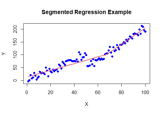Segmented Regression in R

The blue dots represent the data points. The red line represents the first segment of the regression, fitted to the first 50 data points.

Quantile Regression

quantile regression produces estimates of the conditional quantiles of the response variable, such as the median or quartiles. In this respect, it is resistant to outliers; moreover, it offers a capacity for modeling the distribution of the response variable more accurately. Key Concepts in Quantile Regression are:

1. Conditional Quantiles: Quantile regression estimates the relationship between variables for different quantiles (e.g., median, 25th percentile, 75th percentile).
2. Robustness: Quantile regression is more robust to outliers than mean regression since it focuses on medians or other quantiles.
3. Flexibility: It allows for the analysis of the impact of covariates on different points of the outcome distribution.

library(quantreg)
set.seed(123)
x <- rnorm(100)
y <- 2 * x + rnorm(100, 0, 1) + abs(x)
data <- data.frame(x = x, y = y)
rq_50 <- rq(y ~ x, data = data, tau = 0.5)  # Median regression
rq_25 <- rq(y ~ x, data = data, tau = 0.25) # 25th percentile
rq_75 <- rq(y ~ x, data = data, tau = 0.75) # 75th percentile
plot(data$x, data$y, pch = 16, col = "blue", 
     main = "Quantile Regression Example", xlab = "X", ylab = "Y")
abline(rq_50, col = "red", lwd = 2, lty = 1)  # Median regression line
abline(rq_25, col = "green", lwd = 2, lty = 2) # 25th percentile line
abline(rq_75, col = "yellow", lwd = 2, lty = 3) # 75th percentile line
legend("topleft", legend = c("Median (50th percentile)", "25th percentile", 
                             "75th percentile"),
       col = c("red", "green", "yellow"), lwd = 2, lty = 1:3)

Output:

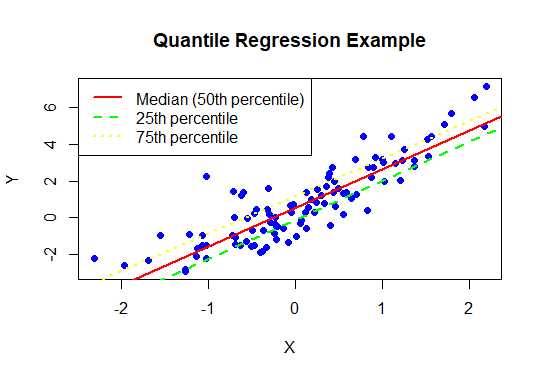Quantile regression in R

• The blue dots represent the data points.
• The red line represents the median regression (50th percentile).
• The green dashed line represents the 25th percentile regression.
• The yellow dotted line represents the 75th percentile regression

Implementation of segmented regression using quantile regression in R

Here’s a step-by-step guide to combining segmented and quantile regression to improve performance:

Step 1: Install and load packages

First we will install the required libraries and load them :

# Installing the Libraries.
install.packages("segmented")
install.packages("quantreg")
# Loading the Libraries.
library(segmented)
library(quantreg)

Step 2: Create data

Next, we will start the process of preparing the data.

# Example data
set.seed(123)
x <- seq(1, 100)
y <- c(rnorm(50, mean = 5), rnorm(50, mean = 10)) + rnorm(100)
data <- data.frame(x, y)
head(data)

Output:

  x        y
1 1 3.729118
2 2 5.026706
3 3 6.312016
4 4 4.722966
5 5 4.177669
6 6 6.670037

Step 3: Fit Initial Linear Model

The first step in fitting an initial linear model would be to generate a simple linear regression model by which baseline information about relationships between variables of interest is established, so one may progress to more complex techniques such as segmented and quantile regression.

linear_model <- lm(y ~ x, data = data)

Step 4: Identify Breakpoints and applying segmented regression

Breakpoints are identified by the points at which there is a huge change or break in the relationship of variables. This is very important for segmented regression where, perhaps, different segments may follow distinctly different regression lines.

segmented_model <- segmented(linear_model, seg.Z = ~ x, psi = list(x = c(50)))

Step 5: Applying Quantile Regression

Quantile regression estimators provide conditional quantiles of the response variable, robust to outliers and non-normality in data.

quantile_model <- rq(y ~ x, tau = 0.5, data = data)

• rq is the function from the quantreg package in R for quantile regression.
• y ~ x specifies the formula where y is the response variable and x is the predictor variable.
• tau = 0.5 specifies the median regression (quantile = 0.5). Adjust tau for different quantiles.

Step 6: Combine Models For Enhanced Performance

The combination of segmented regression with quantile regression increased model performance by using the power of both techniques together.

breakpoints <- segmented_model$psi[, 2]
data$segment <- ifelse(data$x <= breakpoints[1], 1, 2)
combined_model <- rq(y ~ x * segment, tau = 0.5, data = data)

• breakpoints extracts the identified breakpoints from segmented_model.
• ifelse(data$x <= breakpoints[1], 1, 2) assigns segment labels based on breakpoints.
• rq(y ~ x * segment, tau = 0.5, data = data) fits quantile regression within each segment defined by segment.

Step 7: Compare Models

Compare the performance of the basic quantile regression model and the segmented quantile regression model. You can use various criteria such as the Akaike Information Criterion (AIC), Bayesian Information Criterion (BIC), or graphical diagnostics.

# Compare models using AIC
AIC(linear_model, segmented_model,quantile_model)

Output:

                df      AIC
linear_model     3 414.9622
segmented_model  5 412.7035
quantile_model   2 419.7465

• The segmented model has the lowest AIC value (412.7035), indicating it provides the best trade-off between model complexity and goodness of fit among the three models considered.
• The linear model has a slightly higher AIC value (414.9622) than the segmented model, indicating that while it is simpler (lower degrees of freedom), it does not fit the data as well as the segmented model.
• The quantile model has the highest AIC value (419.7465), suggesting it is the least preferred model among the three due to poorer fit to the data.

In summary, when selecting a model based on AIC, the segmented model is preferred over both the linear and quantile models for this dataset, as it offers the best compromise between model complexity and explanatory power.

Step 8: Visualize the Results

Visualize the results to understand the fit and the identified segments:

# Plot original data
plot(data$x, data$y, col = "blue", pch = 19, xlab = "x", ylab = "y", 
                                      main = "Segmented and Quantile Regression")

# Add linear regression line
abline(linear_model, col = "red")

# Add segmented regression lines
segments <- segmented_model$psi[, 2]
abline(v = segments, col = "green", lty = 2)

# Add quantile regression line
lines(data$x, predict(quantile_model, data.frame(x = data$x)), col = "purple")

# Add legend
legend("topleft", legend = c("Data", "Linear Regression", "Segmented Lines", 
                                                                "Quantile Regression"),
       col = c("blue", "red", "green", "purple"), lty = c(NA, 1, 2, 1), 
                                                                pch = c(19, NA, NA, NA))

Output:

segmented regression using quantile regression in R

Conclusion

In using segmented regression with quantile regression in R, analysts are better placed to improve the modeling of complex relationships in data, deal with outliers and heteroscedasticity, and make meaningful inferences from data. Such techniques not only ensure the accuracy and robustness of statistical models but also offer a general framework within which the appraisal and interpretation of patterns found in data can be better done. By merging these methodologies into your analytic toolkit, you’ll be better placed to overcome sophisticated data analysis challenges confidently and to make sure that your models are both rigorous and insightful in their applications.