A decision tree classifier is a well-liked and adaptable machine learning approach for classification applications. It creates a model in the shape of a tree structure, with each internal node standing in for a “decision” based on a feature, each branch for the decision’s result, and each leaf node for a regression value or class label. Decision trees are the fundamental components of random forests.

In this article, we will delve into the world of Decision Tree Classifiers using Scikit-Learn, a popular Python library for machine learning. We will explore the theoretical foundations, implementation, and practical applications of Decision Tree Classifiers, providing a comprehensive guide for both beginners and experienced practitioners.

What is a Decision Tree Classifier?

A Decision Tree Classifier is a type of supervised learning algorithm that uses a tree-like model to classify data into different categories. The algorithm works by recursively partitioning the data into smaller subsets based on the values of the input features. Each internal node in the tree represents a feature or attribute, and each leaf node represents a class label. The classification process involves traversing the tree from the root node to a leaf node, with each node providing a decision based on the input features.

How Does a Decision Tree Classifier Work?

The Decision Tree Classifier algorithm can be broken down into three main steps:

1. Root Node Selection: The algorithm starts by selecting the root node, which represents the entire dataset.
2. Feature Selection: At each internal node, the algorithm selects the most informative feature to split the data. This is typically done using a metric such as information gain or Gini impurity.
3. Splitting: The algorithm splits the data into two subsets based on the selected feature and a threshold value.
4. Recursion: Steps 2 and 3 are repeated recursively until a stopping criterion is reached, such as a maximum depth or a minimum number of samples.

Implementing Decision Tree Classifiers with Scikit-Learn

The DecisionTreeClassifier from Sklearn has the ability to perform multi-class classification on a dataset. The syntax for DecisionTreeClassifier is as follows:

class sklearn.tree.DecisionTreeClassifier(*, criterion=’gini’, splitter=’best’, max_depth=None,  min_samples_split=2, min_samples_leaf=1, min_weight_fraction_leaf=0.0, max_features=None, random_state=None, max_leaf_nodes=None, min_impurity_decrease=0.0, class_weight=None,  ccp_alpha=0.0, monotonic_cst=None)

Let’s go through the parameters:

• criterion: It meeasure the quality of a split. Supported values are ‘gini’, ‘entropy’, and ‘log_loss’. The default value is ‘gini’
• splitter: This param is used to choose the split at each node. Supported values are ‘best’ & ‘random’. The default value is ‘best’
• max_features: It defines the no. of features to consider when looking for the best split.
• max_depth: The max_depth parameter denotes maximum depth of the tree(default=None).
• min_samples_split: It defines the minimum no. of samples reqd. to split an internal node (default=2).
• min_samples_leaf: The minimum number of samples required to be at a leaf node (default=1)
• max_leaf_nodes: It defines the maximum number of possible leaf nodes.
• min_impurity_split: It defines the threshold for early stopping tree growth.
• class_weight: It defines the weights associated with classes.
• ccp_alpha:It is a complexity parameter used for minimal cost-complexity pruning

Steps to train a DecisionTreeClassifier Using Sklearn

Let’s look at how to train a DecisionTreeClassifier using Sklearn on Iris dataset. The phase by phase execution as follows:

Step 1: Import Libraries

To start, import the libraries you’ll need, such as Scikit-Learn (sklearn) for machine learning tasks.

from sklearn.datasets import load_iris
from sklearn.model_selection import train_test_split
from sklearn.tree import DecisionTreeClassifier
from sklearn.metrics import accuracy_score

Step 2: Data Loading

In order to perform classification jobs, load a dataset. For demonstration, one can utilize sample datasets from Scikit-Learn, such as Iris or Breast Cancer.

iris = load_iris()
X = iris.data
y = iris.target

Step 3: Splitting Data

Use the train_test_split method from sklearn.model_selection to split the dataset into training and testing sets.

X_train, X_test, y_train, y_test = train_test_split(X, y, test_size=0.3, random_state=99)

Step 4: Starting the Model

Using DecisionTreeClassifier from sklearn.tree, create an object for the Decision Tree Classifier.

clf = DecisionTreeClassifier(random_state=1)

Step 5: Training the Model

Apply the fit method to match the classifier to the training set of data.

clf.fit(X_train, y_train)

Step 6: Making Predictions

Apply the predict method to the test data and use the trained model to create predictions.

y_pred = clf.predict(X_test)

accuracy = accuracy_score(y_test, y_pred)
print(f'Accuracy: {accuracy}')

Let’s implement the complete code based on above steps. The code is as follows:

from sklearn.datasets import load_iris
from sklearn.model_selection import train_test_split
from sklearn.tree import DecisionTreeClassifier
from sklearn.metrics import accuracy_score

# load iris dataset
iris = load_iris()
X = iris.data
y = iris.target

# split dataset to training and test set
X_train, X_test, y_train, y_test = train_test_split(
    X, y, test_size=0.3, random_state = 99)

# initialize decision tree classifier
clf = DecisionTreeClassifier(random_state=1)
# train the classifier
clf.fit(X_train, y_train)
# predict using classifier
y_pred = clf.predict(X_test)

# claculate accuracy
accuracy = accuracy_score(y_test, y_pred)
print(f'Accuracy: {accuracy}')

Output:

Accuracy: 0.9555555555555556

Hyperparameter Tuning with Decision Tree Classifier

The performance of a decision tree classifier can be greatly impacted by hyperparameters. Tuning hyperparameters can result in increased performance, reduced overfitting, enhanced generalization, etc. Some of the major hyperparameters in a decision tree classifier are criterion, splitter, max_features, max_depth, min_sample_leaf, max_leaf_nodes, etc.

The three most widely used methods for hyperparameter tuning are Grid Search, Random Search and Bayesian optimization. These methods check the different combinations of hyperparameter values that help to find the most effective configuration and fine-tune the decision tree model.

For more details, you can check out the article How to tune a Decision Tree in Hyperparameter tuning?

Hyperparmater tuning using GridSearchCV

Let’s make use of Scikit-Learn’s GridSearchCV to find the best combination of of hyperparameter values. The code is as follows:

from sklearn.model_selection import GridSearchCV

# Hyperparameter to fine tune
param_grid = {
    'max_depth': range(1, 10, 1),
    'min_samples_leaf': range(1, 20, 2),
    'min_samples_split': range(2, 20, 2),
    'criterion': ["entropy", "gini"]
}
# Decision tree classifier
tree = DecisionTreeClassifier(random_state=1)
# GridSearchCV
grid_search = GridSearchCV(estimator=tree, param_grid=param_grid, 
                           cv=5, verbose=True)
grid_search.fit(X_train, y_train)

# Best score and estimator
print("best accuracy", grid_search.best_score_)
print(grid_search.best_estimator_)

Output:

Fitting 5 folds for each of 1620 candidates, totalling 8100 fits 
best accuracy 0.9714285714285715 
DecisionTreeClassifier(criterion='entropy', max_depth=4, 
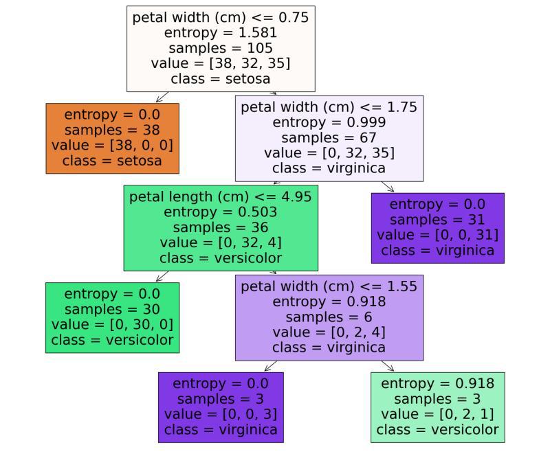
min_samples_leaf=3, random_state=1)

Here we defined the parameter grid with a set of hyperparameters and a list of possible values. The GridSearchCV evaluates the different hyperparameter combinations for the DecissionTree Classifier and selects the best combination of hyperparameters based on the performance across all k folds.

Visualizing the Decision Tree Classifier

Decision Tree visualization facilitates interpretation and comprehension of the model’s choices. We’ll plot feature importances obtained from the Decision Tree model to see which features have the greatest predictive power. Here we fetch the best estimator obtained from the gridsearchcv as the decision tree classifier.

from sklearn.tree import plot_tree
import matplotlib.pyplot as plt

# best estimator 
tree_clf = grid_search.best_estimator_
# plot 
plt.figure(figsize=(18, 15))
plot_tree(tree_clf, filled=True, feature_names=iris.feature_names,
          class_names=iris.target_names)
plt.show()

Output:

DecisionTree Visualization

Let’s look at how trees make predictions based on the above diagram. We can start from the root node (depth 0, at the top). The root node checks whether the flower petal width is less than or equal to 0.75. If it is, then we move to the root’s left child node (depth1, left). Here, the left node doesn’t have any child nodes, so the classifier will predict the class for that node (setosa).

If the petal width is greater than 0.75, then we must move down to the root’s right child node (depth 1, right). Here the right node is not a leaf node, so node check for the condition until it reaches the leaf node.

Decision Tree Classifier With Spam Email Detection Dataset

Spam email detection dataset is trained on decision trees to predict e-mails as spam or ham (safe). As scikit-learn is also known as Sklearn it is used as sklearn library for this implementation

Let’s load the spam email dataset and plot the count of spam and ham emails using matplotlib. The code is as follows:

import pandas as pd
import matplotlib.pyplot as plt

# load dataset
dataset_link = 'https://media.geeksforgeeks.org/wp-content/uploads/20240620175612/spam_email.csv'
df = pd.read_csv(dataset_link)

# plot the category count
df['Category'].value_counts().plot.bar(color = ["g","r"]) 
plt.title('Total number of ham and spam in the dataset') 
plt.show()

Output

Spam and Ham Email Count

As a next step, let’s prepare the data for decision tree classifier. The code is as follows:

from nltk.tokenize import RegexpTokenizer
from sklearn.feature_extraction.text import CountVectorizer
from sklearn.model_selection import train_test_split

def clean_str(string):
    # Clean a string with RegexpTokenizer
    reg = RegexpTokenizer(r'[a-z]+')
    string = string.lower()
    tokens = reg.tokenize(string)
    return " ".join(tokens)

# replace category string with numeric
df['Category'] = df['Category'].map({'ham' : 0,'spam' : 1 })
# clean the message 
df['text_clean'] = df['Message'].apply(
  lambda string: clean_str(string))

# Convert a collection of text documents to a matrix of token counts
cv = CountVectorizer()
X = cv.fit_transform(df.text_clean)

# Get the categories
y = df.Category

# Split training and test dataset
x_train, x_test, y_train, y_test = train_test_split(
    X, y, test_size = 0.2, random_state = 42)

As part of data preparation, the category string is replaced with a numeric attribute, RegexpTokenizer is used for message cleaning, and CountVectorizer() is used to convert text documents to a matrix of tokens. Finally, the dataset is separated into training and test sets.

Now we can use the prepared data to train a DecisionTreeClassifier. The code is as follows:

from sklearn.metrics import (
    accuracy_score, classification_report,
    confusion_matrix)
from sklearn.tree import DecisionTreeClassifier

# Decision Tree Classifier
model = DecisionTreeClassifier()
# train the model
model.fit(x_train, y_train)
# predict using test data
pred = model.predict(x_test)

# Accuracy Metrics
print(classification_report(y_test, pred))

Output:

              precision    recall  f1-score   support              
0                    0.98      0.98      0.98       966            
1                     0.89      0.89      0.89       149       
accuracy                                 0.97      1115    
macro avg   0.94      0.93   0.94          1115  
weighted avg 0.97      0.97      0.97      1115

Here we used DecisionTreeClassifier from sklearn to train our model, and the classicfication_metrics() is used for evaluating the predictions. Let’s check the confusion matrix for the decision tree classifier.

import seaborn as sns

# confusion matrix
cmat = confusion_matrix(y_test, pred)

# plot heatmap
sns.heatmap(cmat, annot=True, cmap='Paired', 
            cbar=False, fmt="d", xticklabels=[
            'Not Spam', 'Spam'], yticklabels=['Not Spam', 'Spam'])

Output:

Heatmap

Advantages and Disadvantages of Decision Tree Classifier

Advantages of Decision Tree Classifier

• Interpretability: Decision trees are accessible for comprehending the decisions made by the model because they are simple to grasp and display.
• Takes Care of Non-linearity: They don’t need feature scaling in order to capture non-linear correlations between features and target variables.
• Handles Mixed Data Types: Without the necessity for one-hot encoding, decision trees are able to handle both numerical and categorical data.
• Feature Selection: By choosing significant features further up the tree, they obliquely carry out feature selection.
• No Assumptions about Data Distribution: Unlike parametric models, decision trees do not make any assumptions on the distribution of data.
• Robust to Outliers: Because of the way dividing nodes works, they are resistant to data outliers.

Drawbacks of Decision Tree Classifier

• Overfitting: If training data isn’t restricted or pruned, decision trees have a tendency to overfit and capture noise and anomalies.
• Instability: Minor changes in the data might result in entirely different tree structures, which is what makes them unstable.
• Difficulty in Capturing Complex interactions: Deeper trees may be necessary in order to capture complex interactions such as XOR.
• Bias towards Dominant Classes: Decision Trees may exhibit bias towards dominant classes in datasets with an uneven distribution of classes.

Conclusion

In this article, we have explored the world of Decision Tree Classifiers using Scikit-Learn. We have covered the theoretical foundations, implementation, and practical applications of Decision Tree Classifiers, providing a comprehensive guide for both beginners and experienced practitioners. By understanding the strengths and limitations of Decision Tree Classifiers, we can harness their power to build accurate and interpretable machine learning models.