Radial Basis Function (RBF) Neural Networks are a specialized type of Artificial Neural Network (ANN) used primarily for function approximation tasks. Known for their distinct three-layer architecture and universal approximation capabilities, RBF Networks offer faster learning speeds and efficient performance in classification and regression problems. This article delves into the workings, architecture, and applications of RBF Neural Networks.

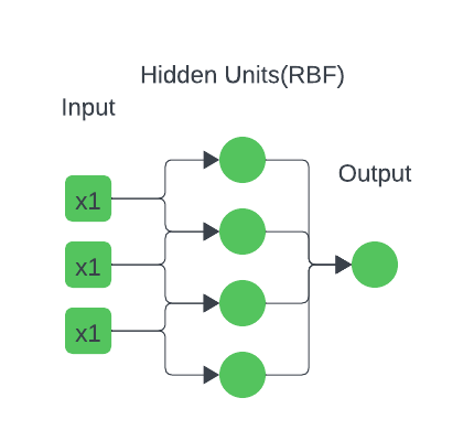
What are Radial Basis Functions?

Radial Basis Functions (RBFs) are a special category of feed-forward neural networks comprising three layers:

1. Input Layer: Receives input data and passes it to the hidden layer.
2. Hidden Layer: The core computational layer where RBF neurons process the data.
3. Output Layer: Produces the network’s predictions, suitable for classification or regression tasks.

How Do RBF Networks Work?

RBF Networks are conceptually similar to K-Nearest Neighbor (k-NN) models, though their implementation is distinct. The fundamental idea is that an item’s predicted target value is influenced by nearby items with similar predictor variable values. Here’s how RBF Networks operate:

1. Input Vector: The network receives an n-dimensional input vector that needs classification or regression.
2. RBF Neurons: Each neuron in the hidden layer represents a prototype vector from the training set. The network computes the Euclidean distance between the input vector and each neuron’s center.
3. Activation Function: The Euclidean distance is transformed using a Radial Basis Function (typically a Gaussian function) to compute the neuron’s activation value. This value decreases exponentially as the distance increases.
4. Output Nodes: Each output node calculates a score based on a weighted sum of the activation values from all RBF neurons. For classification, the category with the highest score is chosen.

Key Characteristics of RBFs

• Radial Basis Functions: These are real-valued functions dependent solely on the distance from a central point. The Gaussian function is the most commonly used type.
• Dimensionality: The network’s dimensions correspond to the number of predictor variables.
• Center and Radius: Each RBF neuron has a center and a radius (spread). The radius affects how broadly each neuron influences the input space.

Architecture of RBF Networks

The architecture of an RBF Network typically consists of three layers:

Input Layer

• Function: After receiving the input features, the input layer sends them straight to the hidden layer.
• Components: It is made up of the same number of neurons as the characteristics in the input data. One feature of the input vector corresponds to each neuron in the input layer.

Hidden Layer

• Function: This layer uses radial basis functions (RBFs) to conduct the non-linear transformation of the input data.
• Components: Neurons in the buried layer apply the RBF to the incoming data. The Gaussian function is the RBF that is most frequently utilized.
• RBF Neurons: Every neuron in the hidden layer has a spread parameter (σ) and a center, which are also referred to as prototype vectors. The spread parameter modulates the distance between the center of an RBF neuron and the input vector, which in turn determines the neuron’s output.

Output Layer

• Function: The output layer uses weighted sums to integrate the hidden layer neurons’ outputs to create the network’s final output.
• Components: It is made up of neurons that combine the outputs of the hidden layer in a linear fashion. To reduce the error between the network’s predictions and the actual target values, the weights of these combinations are changed during training.

Training Process of radial basis function neural network

An RBF neural network must be trained in three stages: choosing the center’s, figuring out the spread parameters, and training the output weights.

Step 1: Selecting the Centers

• Techniques for Centre Selection: Centre’s can be picked at random from the training set of data or by applying techniques such as k-means clustering.
• K-Means Clustering: The center’s of these clusters are employed as the center’s for the RBF neurons in this widely used center selection technique, which groups the input data into k groups.

Step 2: Determining the Spread Parameters

• The spread parameter (σ) governs each RBF neuron’s area of effect and establishes the width of the RBF.
• Calculation: The spread parameter can be manually adjusted for each neuron or set as a constant for all neurons. Setting σ based on the separation between the center’s is a popular method, frequently accomplished with the help of a heuristic like dividing the greatest distance between canters by the square root of twice the number of center’s

Step 3: Training the Output Weights

• Linear Regression: The objective of linear regression techniques, which are commonly used to estimate the output layer weights, is to minimize the error between the anticipated output and the actual target values.
• Pseudo-Inverse Method: One popular technique for figuring out the weights is to utilize the pseudo-inverse of the hidden layer outputs matrix

Here is an example of a Python code implementation that makes use of NumPy:

import numpy as np
from scipy.spatial.distance import cdist

# Generate sample data
np.random.seed(0)
X = np.random.rand(100, 2)
y = np.sin(X[:, 0]) + np.cos(X[:, 1])

# Define the radial basis function
def rbf(x, c, s):
    return np.exp(-np.linalg.norm(x-c)**2 / (2 * s**2))

# Choose centers using k-means
from sklearn.cluster import KMeans
kmeans = KMeans(n_clusters=10).fit(X)
centers = kmeans.cluster_centers_

# Calculate the spread parameter
d_max = np.max(cdist(centers, centers, 'euclidean'))
sigma = d_max / np.sqrt(2 * len(centers))

# Compute the RBF layer output
R = np.zeros((X.shape[0], len(centers)))
for i in range(X.shape[0]):
    for j in range(len(centers)):
        R[i, j] = rbf(X[i], centers[j], sigma)

# Compute the output weights
W = np.dot(np.linalg.pinv(R), y)

# Define the RBF network prediction function
def rbf_network(X, centers, sigma, W):
    R = np.zeros((X.shape[0], len(centers)))
    for i in range(X.shape[0]):
        for j in range(len(centers)):
            R[i, j] = rbf(X[i], centers[j], sigma)
    return np.dot(R, W)

# Make predictions
y_pred = rbf_network(X, centers, sigma, W)

# Evaluate the model
from sklearn.metrics import mean_squared_error
mse = mean_squared_error(y, y_pred)
print(f"Mean Squared Error: {mse}")

Output:

Mean Squared Error: 0.016605403732061076

Advantages of RBF Networks

1. Universal Approximation: RBF Networks can approximate any continuous function with arbitrary accuracy given enough neurons.
2. Faster Learning: The training process is generally faster compared to other neural network architectures.
3. Simple Architecture: The straightforward, three-layer architecture makes RBF Networks easier to implement and understand.

Applications of RBF Networks

• Classification: RBF Networks are used in pattern recognition and classification tasks, such as speech recognition and image classification.
• Regression: These networks can model complex relationships in data for prediction tasks.
• Function Approximation: RBF Networks are effective in approximating non-linear functions.

Example of RBF Network

Consider a dataset with two-dimensional data points from two classes. An RBF Network trained with 20 neurons will have each neuron representing a prototype in the input space. The network computes category scores, which can be visualized using 3-D mesh or contour plots. Positive weights are assigned to neurons belonging to the same category and negative weights to those from different categories. The decision boundary can be plotted by evaluating scores over a grid.

Conclusion

Neural networks with radial basis functions are an effective tool for many different machine learning applications. They can efficiently simulate complex, non-linear interactions thanks to their three-layer architecture, which consists of an input layer, a hidden layer with radial basis functions, and a linear output layer. Choosing the right centres, figuring out the spread parameters, and training the output weights are the steps in the training process. RBF networks provide a flexible and reliable solution for a wide range of real-world issues. They are especially helpful in function approximation, pattern recognition, time-series prediction, and control systems.

Radial Basis Function Neural Networks FAQs

How do you choose the centers in an RBF network ?

The selection of center’s can be done by training via optimization approaches, random selection from the training data, or even k-means clustering. Using the cluster center’s as the RBF center’s, K-means clustering is a well-liked technique that divides the input data into clusters.

What is the spread parameter in an RBF network ?

The radial basis function’s width and the degree to which each center affects the input space are both controlled by the spread parameter (σ). It can be chosen specifically for each RBF neuron or set as a constant for all of them. Determining σ by measuring the distance between center’s is a popular heuristic.

What are the advantages of RBF networks ?

RBF networks have a number of benefits over other neural networks, including as simplicity in design and implementation, flexibility in modelling non-linear connections, and efficiency in training with less data. Additionally, they offer localized replies, which is advantageous in some circumstances.

How are the output weights trained in an RBF network ?

The most common method for training the output weights is linear regression. One popular method is to minimize the error between the anticipated outputs and the actual target values by solving for the weights using the pseudo-inverse of the hidden layer output matrix.

Can RBF networks be used for deep learning ?

The concepts of RBF networks can be applied to deeper designs, even though they are typically shallow networks with a single hidden layer. On the other hand, compared to other neural network types like convolutional neural networks (CNNs) and recurrent neural networks (RNNs), which are specifically made to handle complicated data structures like images, sequences, and other high-dimensional data, they are less frequently utilized in deep learning.