Time series data is ubiquitous in various fields such as finance, meteorology, medicine, and more. Detecting significant changes in time series data is crucial for understanding underlying patterns and making informed decisions. However, it is equally important to determine when these changes are no longer significant. This article delves into the technical aspects of detecting significant changes in time series data and how to ascertain when these changes cease to be significant.

Understanding Change Point Detection

Change point detection (CPD) is a technique used to identify points in time where the statistical properties of a time series change abruptly. These changes can manifest in various forms, such as shifts in mean, variance, correlation, or spectral density. CPD is essential for applications like quality control in manufacturing, climate change analysis, and medical condition monitoring.

Types of Change Points

1. Mean Shift: Detects changes in the average value of the time series.
2. Variance Shift: Identifies changes in the variability of the data.
3. Trend Shift: Detects changes in the slope or linear trend of the data.
4. Frequency Shift: Identifies changes in the periodicity or frequency of the data

Methods for Change Point Detection

Several methods have been developed for detecting change points in time series data. These methods can be broadly categorized into offline and online techniques.

1. Offline Change Point Detection

Offline methods analyze the entire time series data to identify change points. These methods are suitable for post hoc analysis and often provide more accurate estimations of change points.

1. Cumulative Sum (CUSUM): This method detects changes in the mean by accumulating deviations from the mean over time.
2. Bayesian Change Point Detection: Uses Bayesian inference to estimate the probability of change points occurring at different times.
3. Segmentation Algorithms: Divide the time series into segments with distinct statistical properties.

2. Online Change Point Detection

Online methods detect change points in real-time as new data becomes available. These methods are crucial for applications requiring immediate detection of changes.

1. Sequential Analysis: Continuously monitors the data stream and updates the detection statistics in real-time.
2. Streaming Algorithms: Designed to handle large volumes of data and provide quick detection of change points.

Threshold Selection Strategies for Detecting Significant Changes

Selecting an appropriate threshold for detecting significant changes is crucial. This threshold can be fixed or adaptive, depending on the nature of the time series.

• Fixed Threshold: Suitable for stationary time series with stable statistical properties. A common approach is to use a multiple of the standard deviation as the threshold.
• Adaptive Threshold: Necessary for non-stationary time series where the statistical properties change over time. Adaptive thresholds adjust based on the signal-to-noise ratio. suggest heading.

Evaluating the Significance of Change Points

Once change points are detected, it is essential to evaluate their significance. This involves determining whether the detected changes are statistically significant or merely due to random fluctuations. Statistical Tests:

1. Hypothesis Testing: Used to test whether the change points are statistically significant. Common tests include the t-test for mean shifts and the F-test for variance shifts.
2. Bayesian Information Criterion (BIC): A model selection criterion that balances model fit and complexity. Lower BIC values indicate more significant change points.

Detecting When Changes Are No Longer Significant

Determining when changes in time series data are no longer significant involves monitoring the time series for periods of stability. This can be achieved through various techniques:

1. Moving Window Analysis

A moving window analysis involves calculating statistical properties over a sliding window of fixed length. By comparing these properties across different windows, one can identify periods of stability.

1. Moving Average: Smooths the time series by averaging data points within the window. Significant changes are detected when the moving average deviates beyond a threshold.
2. Moving Standard Deviation: Measures the variability within the window. A stable period is indicated when the standard deviation remains low and constant.

2. Control Charts

Control charts are graphical tools used to monitor the stability of a process over time. They plot the time series data along with control limits, which are typically set at ±3 standard deviations from the mean.

1. Shewhart Control Chart: Detects significant changes when data points fall outside the control limits.
2. Exponentially Weighted Moving Average (EWMA) Chart: Provides a more sensitive detection of small shifts by weighting recent data points more heavily.

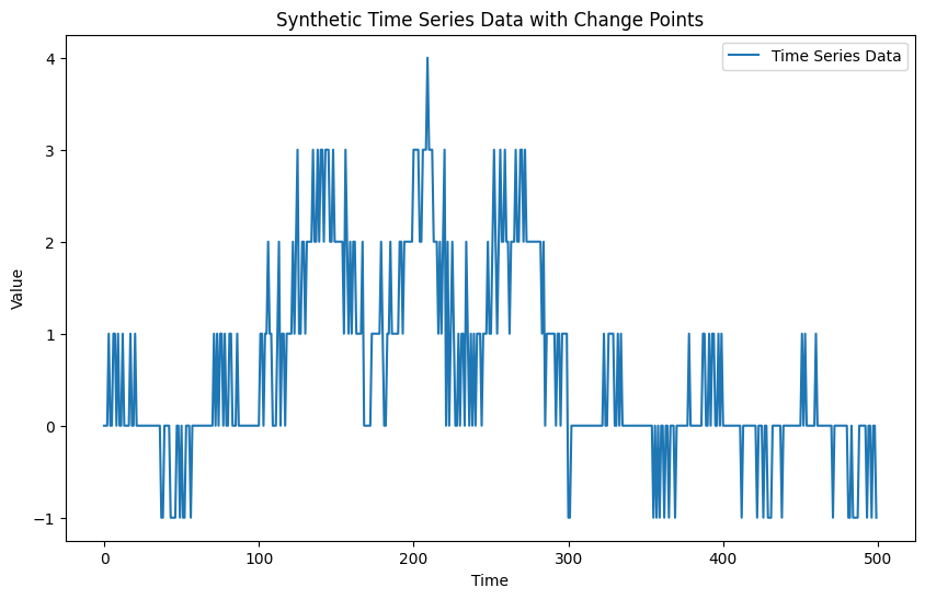
Practical Implementation: Detecting When Changes in Time Series Data Are No Longer Significant

Detecting significant changes in time series data is a crucial task in various fields such as finance, healthcare, and climate science. However, it is equally important to determine when these changes are no longer significant. This practical implementation will guide you through the process using Python, focusing on change point detection and evaluating the significance of these changes.

Step 1: Install and Import Necessary Libraries

!pip install ruptures

First, we need to import the necessary libraries for time series analysis and change point detection.

import numpy as np
import pandas as pd
import matplotlib.pyplot as plt
from ruptures import detect
from statsmodels.tsa.stattools import adfuller

Step 2: Generate or Load Time Series Data

For this example, we will generate synthetic time series data with known change points.

# Generate synthetic time series data
np.random.seed(42)
n = 500
t = np.arange(n)
data = np.piecewise(t, [t < 100, (t >= 100) & (t < 300), t >= 300],
                    [lambda t: np.sin(t / 10) + np.random.normal(0, 0.5, len(t)),
                     lambda t: np.sin(t / 10) + 2 + np.random.normal(0, 0.5, len(t)),
                     lambda t: np.sin(t / 10) + np.random.normal(0, 0.5, len(t))])

# Plot the time series data
plt.figure(figsize=(10, 6))
plt.plot(t, data, label='Time Series Data')
plt.title('Synthetic Time Series Data with Change Points')
plt.xlabel('Time')
plt.ylabel('Value')
plt.legend()
plt.show()

Output:

Time Series Data

Step 3: Detect Change Points

We will use the ruptures library to detect change points in the time series data.

import ruptures as rpt

# Detect change points using the Pelt search method
model = "l2"  # Model for change point detection
algo = rpt.Pelt(model=model).fit(data)
result = algo.predict(pen=10)

# Plot the detected change points
plt.figure(figsize=(10, 6))
plt.plot(t, data, label='Time Series Data')
for cp in result:
    plt.axvline(x=cp, color='r', linestyle='--', label='Change Point' if cp == result[0] else "")
plt.title('Detected Change Points in Time Series Data')
plt.xlabel('Time')
plt.ylabel('Value')
plt.legend()
plt.show()

Output:

Detect Change Points

Step 4: Evaluate the Significance of Change Points

To evaluate the significance of the detected change points, we can use statistical tests such as the Augmented Dickey-Fuller (ADF) test to check for stationarity. The p-values below 0.05, indicates that the null hypothesis of non-stationarity can be rejected. This means that each segment is stationary, and the detected change points are significant.

def adf_test(timeseries):
    result = adfuller(timeseries)
    print('ADF Statistic: %f' % result[0])
    print('p-value: %f' % result[1])
    for key, value in result[4].items():
        print('Critical Values:')
        print(f'   {key}, {value}')

# Evaluate significance of change points
for i in range(len(result) - 1):
    segment = data[result[i]:result[i+1]]
    print(f"Segment {i+1}:")
    adf_test(segment)
    print("\n")

Output:

Segment 1:
ADF Statistic: -2.210469
p-value: 0.202468
Critical Values:
   1%, -3.661428725118324
Critical Values:
   5%, -2.960525341210433
Critical Values:
   10%, -2.6193188033298647


Segment 2:
ADF Statistic: -3.434827
p-value: 0.009827
Critical Values:
   1%, -3.639224104416853
Critical Values:
   5%, -2.9512301791166293
Critical Values:
   10%, -2.614446989619377


Segment 3:
ADF Statistic: -3.929395
p-value: 0.001829
Critical Values:
   1%, -4.223238279489106
Critical Values:
   5%, -3.189368925619835
Critical Values:
   10%, -2.729839421487603


Segment 4:
ADF Statistic: -6.412650
p-value: 0.000000
Critical Values:
   1%, -3.639224104416853
Critical Values:
   5%, -2.9512301791166293
Critical Values:
   10%, -2.614446989619377


Segment 5:
ADF Statistic: -5.653803
p-value: 0.000001
Critical Values:
   1%, -3.639224104416853
Critical Values:
   5%, -2.9512301791166293
Critical Values:
   10%, -2.614446989619377


Segment 6:
ADF Statistic: -4.740883
p-value: 0.000070
Critical Values:
   1%, -3.4615775784078466
Critical Values:
   5%, -2.875271898983725
Critical Values:
   10%, -2.5740891037735847

Step 5: Detect When Changes Are No Longer Significant

To detect when changes are no longer significant, we can use a moving window analysis to monitor the stability of the time series.

We performed a moving window analysis to monitor the stability of the time series. The moving average and moving standard deviation were calculated using a window size of 50.

window_size = 50
moving_avg = np.convolve(data, np.ones(window_size)/window_size, mode='valid')
moving_std = np.array([np.std(data[i:i+window_size]) for i in range(len(data) - window_size + 1)])

# Plot moving average and moving standard deviation
plt.figure(figsize=(10, 6))
plt.plot(t[window_size-1:], moving_avg, label='Moving Average')
plt.plot(t[window_size-1:], moving_std, label='Moving Standard Deviation')
plt.axhline(y=np.mean(moving_std), color='r', linestyle='--', label='Mean Std Dev')
plt.title('Moving Window Analysis')
plt.xlabel('Time')
plt.ylabel('Value')
plt.legend()
plt.show()

Output:

Detect When Changes Are No Longer Significant

The moving average remains relatively stable, with noticeable shifts at the change points.

• The moving standard deviation shows higher variability around the change points, indicating significant changes in the time series.
• After the change points, the standard deviation stabilizes, suggesting that the changes are no longer significant.

The mean standard deviation line helps to identify periods of stability. When the moving standard deviation is close to the mean standard deviation, it indicates that the time series is stable and changes are no longer significant.

Conclusion

Detecting significant changes in time series data and determining when these changes are no longer significant are critical tasks in various fields. By leveraging techniques such as moving window analysis, control charts, and statistical tests, one can effectively monitor time series data for periods of stability. Despite the challenges, ongoing research and advancements in change point detection methods continue to improve our ability to analyze and interpret time series data.