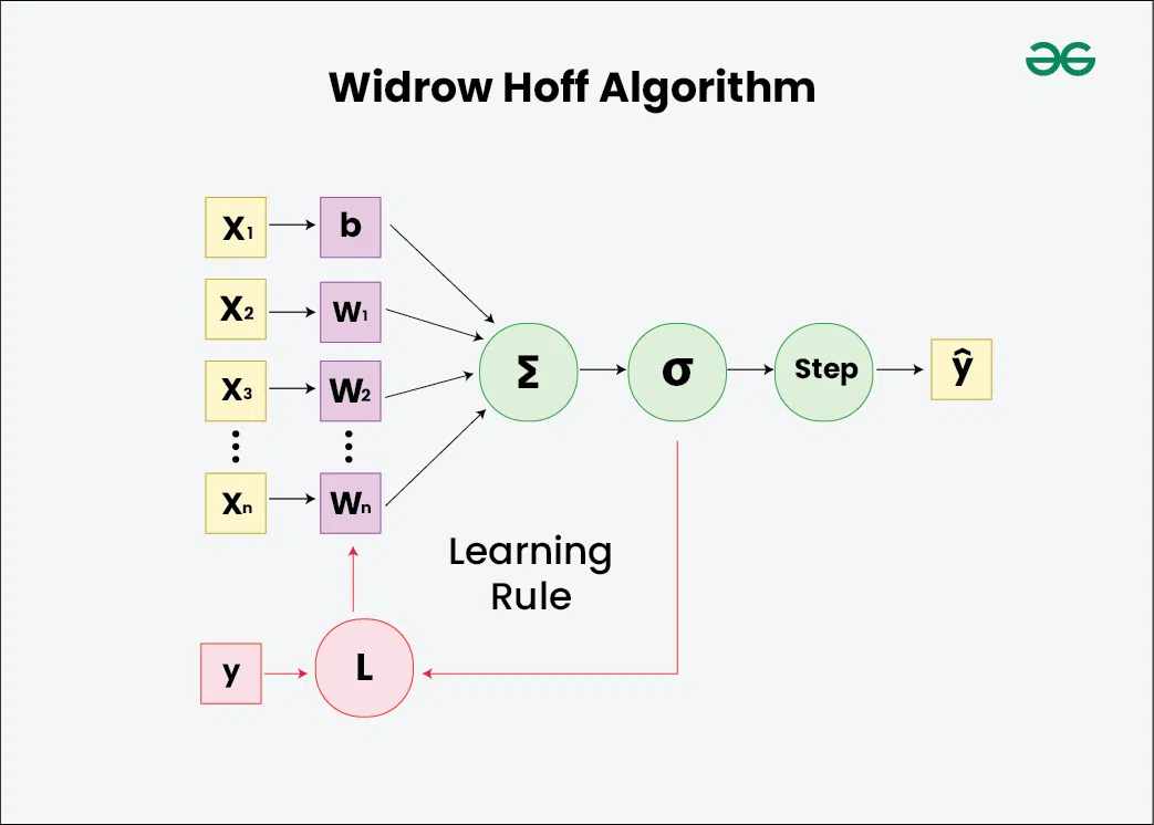
Widrow-Hoff Algorithm is developed by Bernard Widrow and his student Ted Hoff in the 1960s for minimizing the mean square error between a desired output and output produce by a linear predictor. The aim of the article is explore the fundamentals of the Widrow-Hoff algorithm and its impact on the evolution of learning algorithms.

Understanding Widrow-Hoff Algorithm

Widrow-Hoff Learning Algorithm, known as the Least Mean Squares (LMS) algorithm, is used in machine learning, deep learning, and adaptive signal processing. The algorithm is primarily used for supervised learning where the system iteratively adjusts the parameters to approximate a desired target function. It operates by updating the weights of the linear predictor so that the predicted output converges to the actual output over time.

Weight Update Rule in Widrow-Hoff Rule

The update rule guides how the weights of Adaptive Linear Neuron (ADALINE) are adjusted based on the error between expected output and observed output. The weight update rule in the Widrow-Hoff algorithm is given by:

[Tex]w(t+1)=w(t)+η(d(t)−y(t))x(t)[/Tex]

Here,

• [Tex]w(t) [/Tex]and [Tex]w(t+1)[/Tex] are the weight vectors before and after the update, respectively.
• η is the learning rate, a small positive constant that determines the step size of the weight update.
• [Tex]d(t)[/Tex] is the desired output at time t.
• [Tex]y(t) [/Tex]is the predicted output at time t.
• [Tex]x(t)[/Tex] is the input vector at time t.

Interpretation

• Error Signal: [Tex]d(t)−y(t) [/Tex]calculates the error. Positive error means actual output needs to increase, negative means decrease.
• Learning Rate: η scales the error for weight update. A larger error will result in a bigger adjustment to the weights.
• Direction of Update: [Tex]x(t)[/Tex] dictates weight update direction. Positive error adjusts weights in input direction, negative adjusts in opposite direction.

Working Principal of Widrow-Hoff Algorithm

The key steps of the Widrow-Hoff algorithm are:

1. Initialization: Initialize weights randomly.
2. Iterative Update:
   • Compute the predicted output by taking the dot product of the input features and the current weights.
   • Calculate the error between the predicted output and the true output.
   • Update the weights by adding the learning rate multiplied by the error and the input features (gradient descent step).
3. Convergence: Repeat step 2 for multiple epochs or until convergence.

Implementing Widrow-Hoff Algorithm for Linear Regression Problem

We will implement Widrow-Hoff (or LMS) learning algorithm using Python and NumPy to learn weights for a linear regression model, then apply it to synthetic data and print the true weights alongside the learned weights. We have followed these steps:

Step 1: Define the Widrow-Hoff Learning Algorithm

The widrow_hoff_learning function takes the input features (X), target values (y), learning rate, and number of epochs epochs. It initializes random weights, iterates over the dataset for the specified number of epochs, calculates predictions, computes errors, and updates the weights using the Widrow-Hoff update rule.

# Define the Widrow-Hoff (LMS) learning algorithm def widrow_hoff_learning(X, y, learning_rate=0.01, epochs=100): num_features = X.shape[1] weights = np.random.randn(num_features) # Initialize weights randomly for _ in range(epochs): for i in range(X.shape[0]): prediction = np.dot(X[i], weights) error = y[i] - prediction weights += learning_rate * error * X[i] return weights

Step 2: Generate Random Dataset

Random data is generated using NumPy. X is a matrix of 100 samples with 2 features. true_weights represent the true weights used for generating y. Noise is added to y to simulate real data.

# Generate some synthetic training data np.random.seed(0) X = np.random.randn(100, 2) # 100 samples with 2 features true_weights = np.array([3, 5]) # True weights for generating y y = np.dot(X, true_weights) + np.random.randn(100) # Add noise to simulate real data

Step 3: Add a Bias Term

A bias term (constant feature) is added to the feature matrix X to account for the intercept term in the linear model.

# Add a bias term (constant feature) to X X = np.concatenate([X, np.ones((X.shape[0], 1))], axis=1)

Step 4: Apply the Widrow-Hoff Algorithm to learn weights

The widrow_hoff_learning function is called with the generated data X and y to learn the weights.

# Apply the Widrow-Hoff algorithm to learn weights learned_weights = widrow_hoff_learning(X, y)

Complete Implementation of Widrow-Hoff Algorithm for Linear Regression Problem

Output:

True Weights: [3 5] Learned Weights: [3.06124683 5.09292019 0.03074168]

Applications of Widrow-Hoff Algorithm

1. Adaptive Filtering: Widrow-Hoff is used in systems for reducing unwanted noise or interference and enhancing the desired signal.
2. Pattern Recognition: Widrow-Hoff assists in categorizing input data into defined groups based on their features.
3. Signal Processing: Widrow-Hoff is helpful where signals are distorted or have different conditions.