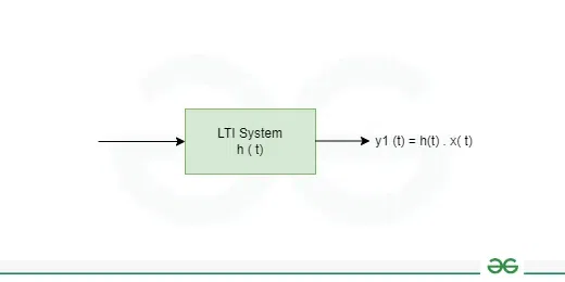
Systems that are both linear and time-invariant are known as linear time-invariant systems, or LTI systems for short. When a system’s outputs for a linear combination of inputs match the outputs of a linear combination of each input response separately, the system is said to be linear. Time-invariant systems are ones whose output is independent of the timing of the input application. Long-term behavior in a system is predicted using LTI systems. The term “linear translation-invariant” can be used to describe these systems, giving it the broadest meaning possible. The analogous term in the case of generic discrete-time (i.e., sampled) systems is linear shift-invariant.

What is a Linear Time Invariant System?

The systems that are both linear and time-invariant are called LTI Systems. The system must be linear and a Time-invariant system. Linear systems have the trait of having a linear relationship between the input and the output. A linear change in the input will also result in a linear change in the output.

In many significant physical systems, these features hold (exactly or approximately), in which case convolution can be used to find the system’s response, y(t), to any given input, x(t). y(t) = (x ∗ h)(t), where ∗ denotes convolution and h(t) is the system’s impulse response

LTI System

For Continuous Signal

Y(t)=∫^∞_−∞h(α)X(t−α)dα=∫^∞_−∞X(α)h(t−α)dα.

In case of discrete signal integration changes to Sigma ( Σ ).

then formula will be,

y[n] = Σ h[α] x[t-α]

where α range -infinity to + infinity

Where ,

x(t) -> input signal

y(t) -> output signal

h(t) -> transfer function

Linear System

If input x₁(t) produces y₁(t) as output and input x₂(t) produces y₂(t) output, then if the combination of the x₁(t) + x₂(t) will produce the y₂(t) + y₂(t) as output then the system is called as the Linear system.

if,

x₁(t) -> y₁(t),

x₂(t) -> y₂(t)

Let x₃(t) = x₁(t) + x₂(t)

Linear system

x₃(t) -> y₃(t) , y₃(t) = y₁(t) + y₂(t)

if satisfied the following condition then system called as linear system.

Time-Invariant System

The output signal are different for the different time shift of the signal called called Time-invariant system. suppose x(t) produce output y(t)

x(t) -> y(t)

and shift in time t -> t + t₀

x(t + t₀) -> y(t + t₀)

Time-invariant system

same for the t -> t – t₀

x(t – t₀) -> y(t – t₀)

x[n] -> y[n]

x[n – n₀] -> y[n – n₀] for( discrete system )

then if the system satisfied following condition called time-invariant system and if the system follow the time-invariant and linear system property then system is called as the linear time-invariant system (LTI).

Homogeneity Principle

If scaling any input signal X(t) also scales the output signal by the same factor, then the system is said to be homogeneous. If x(t) produce the output y(t), Now if the X(t) scale by the factor of the “a” so the respective output also scaled by factor of “a” . As shown in below figure.

Homogeneous system

Superposition Principle

Its define only for the linear system, if input given to the system is x1(t) , x2(t) and output y1(t) , y2(t) respectively. now x1(t) + x2(t) and the output is y1(t) + y2(t).

for continuous-time linear system,

ay1(t) + by2(t) = a[x1(t)] + b[x2(t)]

for discrete-time linear system,

ay1[n] + by2[n] = a[x1[n]] + b[x2[n]]

Types of LTI System

The types of LTI System are mentioned below:

• Continuous-Time LTI Signal
• Discrete Time LTI Signal

Continuous-Time LTI Signal

The impulse response is always taken into account while evaluating LTI systems. In other words, the impulse signal is the input and the impulse response is the output.

here x(t) = δ(t),

and the impulse response the respective output signal is y(t) = h(t) = T. δ(t)

Continuous-time LTI system

Any signal can be described as a combination of a weighted and shifted impulse signal, according to the shifting property of signals.

x(t)=∫^∞_−∞x(τ).δ(t−τ)dτ

the impulse response is,

y(t) = T[x(t)] = ∫^∞_−∞x(τ) . T[δ(t−τ)]dτ,

y(t) = ∫^∞_−∞x(τ) h(t−τ) dτ

from here we got an equation,

y(t) = x(t) ✲ h(t)

Discrete-Time LTI System

In case of discrete time signal ‘t‘ going to replace by the ‘n‘ , here

x[n] = δ(n)

the discrete time input response is given by,

y[n] = h(n) = T δ(n)

Discrete time LTI

Any signal can be described as a combination of a weighted and shifted impulse signal, according to the shifting property of signals.

x[n]=∑ x[k] δ[n−k] where k= [−∞, ∞]

the impulse response y[n] = T δ[n]

y[n] = ∑ x[k]. T[δ(n−k)]

y[n] = ∑ x[k] h[n−k]

so the final output will be,

y[n] = x[n] ✲ h[n]

Properties of LTI System

The unit impulse response of an LTI system can be used to express it in continuous time. It is represented by an integral convolution. Therefore, the LTI system also adheres to the same properties as the continuous time convolution. The significance of an LTI system’s impulse response lies in its ability to fully define its properties.

The property types of LTI system are as follows:

• Invertible System
• Causality
• Commutative Property
• Distributive Property
• Associative Property

These properties of the LTI System are explain below in detail:

• Invertible Systems : If we can determine h(t) such that the output y(t) can be used to recover the original input x(t), then the system is invertible. This requires a one-to-one system in order to hold true.

Invertible System

• Causality : As far as we are aware, a causal system’s output is only dependent on its past or current inputs—it is not dependent on its future inputs. Similarly, an output in a causal system is not dependent on the future; rather, it reacts to an input only after it happens. Put otherwise, a reaction to an input at t = t0 would only happen for t >= t0 and not earlier.

h(t)=0; for t<0

So the equation of y(t) will be,

Output of the causal LTI for non causal input signal.

y(t) = ∫^∞₀h(τ) x(t−τ) dτ = ∫^t_−∞x(τ) h(t−τ) dτ

x(t) -> non causal input signal.

Output of a causal LTI for causal input signal.

y(t) = ∫^t₀ h(τ) x(t−τ) dτ = ∫^t₀ x(τ).h(t−τ) dτ

h(t) -> Transfer function

X(t) -> causal Input signal

• Commutative Property : The convolution of the continuous-time signal is called commutative property.

x(t) ❇ h(t) = h(t) ❇ x(t)

∫^∞_−∞x(τ) . h(t−τ)dτ = ∫^∞_−∞h(τ) x(t−τ)dτ

The output of an LTI system with input x(t) and unit impulse response h(t) is the same as the output of an LTI system with input h(t) and impulse response x(t), given the commutative property of LTI systems.

x(t) -> Input signal.

• Distributive Property: Regarding system connectivity, the distributive property of the LTI system has a helpful meaning. This means that a single system with the impulse response [h₁(t)+h₂(t)] can take the place of the two LTI systems with the impulse responses h1(t) and h2(t) linked in parallel.

x(t) ❇ {h1(t) + h2(t)} = x(t) ❇ h1(t) + x(t) ❇ h2(t)

This is a complex convolution can be divided into multiple simpler convolutions using the distributive property of continuous-time convolution.

Associative Property : According to the given property on changing the order of the signal their will be no change in the convolution, As shown below.

x(t) ❇ [h1(t) ❇ h2(t)] = [x(t) ❇ h1(t)] ❇ h2(t)

Transfer Function of LTI system

A continuous-time LTI system’s transfer function can be defined via the Fourier or Laplace transforms. Further more, the LTI system’s transfer function can only be defined with zero initial circumstances. The transfer function of the LTI system is described in detail in s – domain as well as in frequency domain as follows:

Transfer function

In Frequency Domain

Assuming that the initial conditions are zero, the ratio of the output signal’s Fourier transform to the input signal’s Fourier transform is the transfer function of an LTI system.

Mathematically, transfer function in frequency domain is defined as

H(ω) = Y(ω) / X(ω) ;

suppose if H(ω) is complex then this will be written in the magnitude and phase,

H(ω) = |H(ω)| ejθ(ω) ;

Magnitude response is defined as the |H(ω)| and the phase response θ(ω) = ∠H(ω)

Frequency response of the output,

Y(ω)= X(ω) . H(ω)

Output magnitude = |X(ω)| |H(ω)|

output phase = ∠Y(ω) = ∠H(ω) + ∠X(ω)

In S Domain

When the initial conditions are zero, the ratio of the output signal’s Laplace transform to the input signal’s Laplace transform is the transfer function of the LTI system. Alternatively, when the beginning circumstances are disregarded, the transfer function is defined as the ratio of output to input in the s-domain.

the mathematically explained as the,

H(s) = Y(s) / X(s)

here, The inverse Laplace transform of the transfer function yields the impulse response ℎ(t) of the LTI system in the s-domain.

h(t) = L^-1 [H(s)]

Once an LTI system’s transfer function in the s-domain H(s) is known, determining the transfer function in the frequency domain H(s) only requires changing s in jω.

H(ω) = H(s) |_{s = jω}

jω -> in complex domain.

Convolution

A mathematical technique called convolution can be used to combine two signals into a third signal. Convolution is therefore crucial to signals and systems since it links the input signal with the system’s impulse response to generate the output signal. To put it another way, an LTI system’s input-output relationship is expressed by convolution.

h(t) = T.[δ(t)]

for signal, x(t)

x(t)=∫^∞_−∞x(τ).δ(t−τ)dτ

Convolution Theorem

A system at rest (zero initial conditions) responds to any input by means of the convolution of that input and the system impulse response, according to the main convolution theorem.

let x₁(t), x₂(t) are the two signal then the convolution of the signal is defined as the

x(t) = x₁(t) ✻ x₂(t)

x(t) = ∫^∞_−∞ x₁(T) . x₂(t-T) dτ , −∞ < t < ∞

• Averaging : A moving average, which is a type of convolution, is frequently employed in time series analysis to reduce noise in data by substituting the average of nearby values in a moving window for a given data point. Since a moving average highlights a deeper underlying trend by eliminating short-term variations, it can be thought of as a low-pass filter.
• Smoothing : The process of smoothing aims to highlight long-term trends by removing short-term fluctuations from a signal. For instance, if you plotted a stock’s price changes every day, it would appear noisy; using a smoothing operator may make it clearer if the price was generally rising or falling over time.
• Basic Identity : It is easy to determine the first identity. Let f and g be two functions, and let α be a constant.

[αf ]✻g = f✻[αg] = α[ f✻g ]

Properties of Convolution

We have some basic property that help to reduce the complex calculation.

• Commutative Property: According to this property, the order in which two signals are convolved does not affect the outcome. x₁(t), x₂(t) is the input signal.

x₁(t) ✻ x₂(t) = x₂(t) ✻ x₁(t)

• Distributive Property: If there is a three signal x₁(t), x₂(t) and x₃(t) then distributive property satisfied the following condition.

x₁(t) ✻ [x₂(t) + x₃(t)] = [x₁(t) ✻ x₂(t)] + [x₁(t) ✻ x₃(t)]

• Associative Property: According to the convolution’s associative property, the arrangement of the signals within a convolution has no bearing on the outcome.

[f₁(t) ✻ f₂(t)] ✻ f₃(t) = f₁(t) ✻ [f₂(t) ✻ f₃(t)]

f₁(t), f₂(t) and f₃(t) are the signals

• Invertibility Property: if the x(t) is the signal then passes through the LTI system whose transfer function is h(t), then the output is passed through the another response whose transfer function is set to that level so we get x(t) as output.

so,

Invertible system

h(t) ✻ h1(t) = δ(t)

so the equivalent transfer function is δ(t) so we get x(t) -> x(t).

h1(t), h2(t) are the transfer function.

x(t) -> input signal.

Sampling Theorem

When the sampling frequency fs is larger than or equal to twice the highest frequency component of the message signal, a continuous time signal can be represented in its samples and retrieved.

fs ≥ 2fm

f_m-> is band limit frequency

f_s -> sampling frequency

Let consider a signal x(t) and the impulse train δ(t – nTs)

Input signal

impulse train -> δ(t – nTs)

Impulse Train

now Y(t) = x(t) . δ(t – nTs) …… eq 1

Sampled signal

taking Fourier transform of the first equation.

Y_s(f) = X(F) ✻ F_s Σ δ(f – nf_s)

Y_s(f) = f_s Σ X(f – nf_s)

on plotting the following Ys(f) with frequency.

Output signal

Here, to avoid the overlapping and to get perfect sample :

fs ≥ 2fm .

Aliasing and Anti-Aliasing

When the fs < 2fm then overlapping of the sampling takes place called Aliasing effect. An anti-aliasing filter eliminates any potential under-sampled frequencies from the signal by examining the user-specified sampling frequency.

Aliasing effect

Nyquist Rate

The Nyquist rate of sampling is the lowest theoretical sampling rate at which a signal can be captured and yet be able to be reconstructed from its samples without distortion.

we know that :

f_s = 2f_m

and Nyquist rate T_s = 1 / f_s

Nyquist Interval: The time difference between any two consecutive samples is known as the Nyquist interval when the sampling rate equals the Nyquist rate. The equation is shown below ,

Nyquist Interval = 1 / f_s = 1 / 2f_m

Conclusion

Control theory, signal processing, and filter design, electrical circuit analysis and design, and LTI system theory are all directly related fields of applied mathematics. That is why power plant models are frequently created using them. Electrical circuits are a major application of LTI systems. These circuits, which consist of resistors, transistors, and inductors, form the foundation of contemporary technology. In image processing, where the systems include spatial dimensions instead of or in addition to a temporal dimension, linear time-invariant system theory is also applied. This is also used to determine the long term behavior of any system or device .

FAQs on LTI System

What is the Use of LTI system?

The main purpose of LTI is to facilitate a smooth integration between an external online tool and the learning platform. LTI offers a method that lets users—like students—move between different technologies while upholding a high standard of security for exchanging information about the person, their origins, and their role—like instructor, student, TA, etc

Explain Sampling theorem .

When the sampling frequency fs is larger than or equal to twice the highest frequency component of the message signal, a continuous time signal can be represented in its samples and retrieved.

fs ≥ 2fm

fm-> is band limit frequency

fs -> sampling frequency

Explain nyquist rate.

Two times the frequency that needs to be precisely measured is the Nyquist rate. One can apply the theorem in reverse. At half the sample rate, the Nyquist frequency is the greatest frequency that equipment of that particular sample rate can measure with any degree of reliability.

What do understand form the word convolution in signal and system?

A mathematical method for mixing two signals to create a third is called convolution. In digital signal processing, it is the single most significant approach. Systems are described by a signal known as the impulse response through the use of the impulse decomposition approach.