How to Add Time in Google Sheets- Quick Steps

1. Open your Google Sheets document.
2. Click on the cell where you want to insert the time.
3. Type the time in the desired format (e.g., 3:30 PM).
4. Press Enter, and the time will be inserted into the cell.

Time management is crucial, both in daily life and in spreadsheet mastery. In the dynamic world of spreadsheet management, Google Sheets stands out as a powerful tool for data manipulation and analysis. While basic arithmetic operations are straightforward to perform, dealing with date and time can be a bit tricky.

How to Insert Date and Time in Google Sheets

Step 1: Open Google Sheets and Select Cell

Open your Google Sheets and select the cell where you want to begin by entering the date and time.

Note: Date and time formats depend on the default locale of your spreadsheet , so make sure to change it before you begin .To change it, go to File > Settings. You will see a pop-up window where you can set your region under the General tab > Locale , a drop down menu pops up , select your region . This step will ensure those date and time formats you’re accustomed to.
 

Go to File > Settings

Select your Region and Click on Save Settings

Go to General tab > Locale

Step 2: Select a Method

There are three simple ways to insert date and time into your Google Sheets :

1. Add date and time manually
2. Make Google Sheets auto-populate your column with the date or time
3. Use key combinations to insert the current date and time

How to Add Date and Time Manually in Google Sheets

Note :

• No matter how you want the time to look like at the end, you should always enter it with a colon. This is essential for Google Sheets to distinguish between time and numbers.
• By defaults Google Sheets follows the 24-hour format .
• This is the simplest way to insert date and time into your Google Sheets .

Step 1: Open Google Sheets and Select Cell

Open your Google Sheets and select the cell where you want to add the date/time.

Step 2: Enter the date or time in the cell

Type the time in HH:MM:SS format or the date in DD/MM/YYYY format.

Note :

• Depending on whether you want to represent a clock time or an amount of time , you should use the Time or Duration format, respectively.
• As you all know, the American date format differs from the European one. If you set “United States” as your locale and type in the date in the European format: dd/mm/yyyy, it simply won’t work. The entered date will be treated as a textual value. So, pay attention to that.

Time Format

Google Sheets features different time formats so that you can select one of your choices from hours, minutes, and seconds. To set the time format, select the relevant cells and go to Format > Number>Time.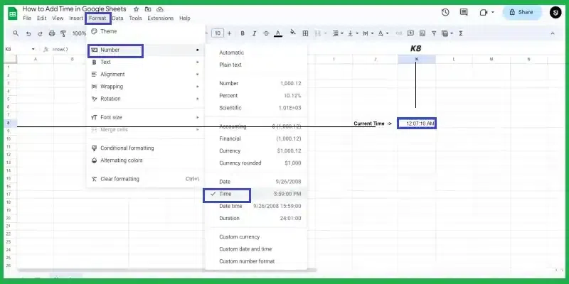
 

Time Format

Duration Format

To set the duration format, select the relevant cells and go to Format > Number > Duration.
 

Duration Format

When working with the duration format, Google Sheets understands integers as days. In other words, One is equal to twenty-four hours: 1 = 24 hours. To represent shorter periods of time, you can use the corresponding fractions.

• 1 hour = 1/24
• 1 minute = 1/(24*60)
• 1 second = 1/(24*60*60)

For example , 5 hours = 5/24 , 3 hours – 30 minutes = ( (3/24) + (30/(24*60)) ) and 1 hour – 50 minutes – 30 seconds = ( (1/24) + (50/(24*60)) + ( 30/(24*60*60) ) ) .Alternatively, you can also use the duration syntax to specify the amount of time: HH:MM:SS. For example, 1 hour – 1 minutes – 1 seconds = 01:01:01.

Alternatively you may type @ in the required cells and continue with the word date and hit enter . A calendar will pops up , set your required date on it . For time use the formula as =TIME(hour, minute, second) and hit enter.

Adding date manually

Similarly, you can add today’s date much quicker. Just type @ in the required cells continue with the word today and hit enter. Google Sheets will recognize your prompt as Today’s date.

How to Make Google Sheets Auto-Populate your Column with Date or Time

Adding time manually

Step 1: Open Google Sheets and Select Cells

Fill in a few cells with the required date time or date time values.

Step 2: Select the cells with the data

Select these cells so you can see a small circle at the bottom right corner of the selection. 

Look for a small circle

 Step 3: Click and Drag the Bottom Right Circle

Click that circle and drag the selection down, covering all required cells.

Step 4: Preview the Result

See how Google Sheets automatically populates those cells based on the two samples you provided, retaining the intervals. Given below is an example with time values, you may similarly do with date values. 
 

How to Use Shortcut Keys to Add Current Date and Time

Step 1: Open Google Sheets and Select Cell

Place the cursor into the cell and press one of the following shortcuts :

1. Ctrl + ; (semicolon) to enter the current date.
2. Ctrl + Shift + ; (semicolon) to enter the current time.
3. Ctrl + Alt + Shift + ; (semicolon) to add both, current date and time.

Step 2: Press the enter key

Use the above shortcuts in the cell and hit the enter key to apply those. Later you’ll be able to edit the values.

This method helps you bypass the problem of entering an incorrect date/time format.

Take advantage of Google Sheets’ date and time functions

• TODAY() — returns the current date to a cell.
• NOW() — returns the current date and time to a cell.
• SPLIT(“<Cell name>” , ” “) — splits the date & time into separate cells.
• HOUR(<Cell name>) — returns the hour component of the specific time.
• MINUTE(<Cell name>) — returns the minute component of the specific time.
• SECOND(<Cell name>) — returns the second component of the specific time.
• TIME VALUE(<Cell name>) — returns the specific time as a fraction of a day 
   

How to Use Excel Data Validation for Entering Dates

Step 1: Open Google Sheets

Go to Data > Data validation in the Google Sheets menu.

Step 2: Set Data validation rules

For dates, just set them as criteria on the range of cells and choose the option that suits you best.
 

Date validation

• For time units, since they are absent from these settings by default, you will need to either create an additional column with time units and refer to this column with your Data validation criteria (List from a range) or enter time units directly to the criteria field (List of items) separating them by a comma.

Time validation

How to Insert Time to Google Sheets in a Custom Number Format

Step 1: Open Google Sheets and Select Cell

For example, you want to add time in minutes and seconds say 12 minutes, 50 seconds. Select any cell say A2 and type 12:50 and press Enter on your keyboard.

Note. No matter how you want the time to look like at the end, you should always enter it with a colon. This is essential for Google Sheets to distinguish between time and numbers.

What you will see is Google Sheets treating your value as 12 hours 50 minutes. If you apply the Duration format to A2, it will still show the time as 12:50:00. So how can you make Google spreadsheet return only minutes and seconds? It is simple, type 00:12:50 into your cell. To be honest, this one may turn out a tiresome process if you need to enter multiple timestamps with minutes and seconds only.

Step 2: Alternative to step 1

• Type 12:50 to A2 cell and put the following formula into A3 as =A2/60
• Apply the Duration number format to A3. Otherwise, your table will always return 12 hours AM.
• Use special formulas. Input minutes to A1, seconds to B1. Enter the following formula to C1 as =TIME(0,A2,B2)

Step 3: Create your own Custom date and time format

In order to delete excess symbols from our time, set the format again. Go to Format>Number>Custom date and time and create a format that will show only elapsed minutes and seconds.
 

Custom date and time

The TIME function refers to cells, takes the values, and transforms them into hours (0), minutes (A1), and seconds (B1).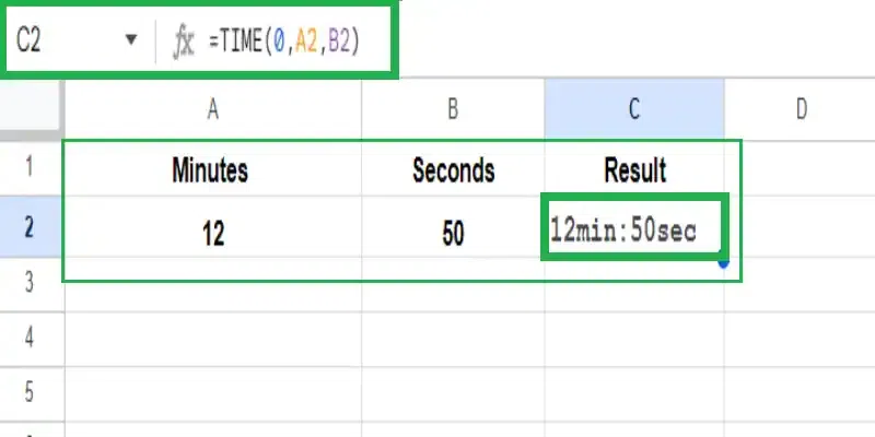

Using TIME function

How to Convert Time to Decimal in Google Sheets

There may be cases when you need to display time as a decimal rather than “HH:MM: SS” to perform various calculations. This is useful in in case you want to count per-hour salary since you can’t perform any arithmetic operations using both, numbers and time. But the problem disappears if time is decimal.

Step 1: Open Google Sheets and Select Cell

Fill the cells with some data you need to work with. Let’s say column A contains the time you started working on some task and column B shows the end time. You want to know how much time it took, and for that, in column C you use the formula as =B2-A2

Step 2: Converting Time to Decimal

Copy the formula down cells C3:C5 and get the result in hours and minutes. Then transfer the values to column D using this formula as =$C2. Then select the entire column D and go to Format > Number > Number.

Step 3: Modify the Time in Decimal

Unfortunately, the result you’ll get at first won’t say much. But Google Sheets has a reason for that: it displays time as a part of a 24-hour period. In other words, 50 minutes is 0.034722 of 24 hours. Of course, this result can be used in calculations. But since we’re used to seeing time in hours, you may want to introduce more calculations to your table.

To be specific, multiply the number you’ve got by 24 (24 hours).

Now you have a decimal value, where integer and fractional reflect the number of hours. To put it simply, 50 minutes is 0.83 hours, while 1 hour 30 minutes is 1.50 hours.

Text-formatted dates to date format with Power Tools for Google Sheets

There’s one quick method for converting dates formatted as text to a date format. It’s called Power Tools. Power Tools is an add-on for Google Sheets that allows you to convert your information in a couple of clicks.

Step 1: Get the add-on for your spreadsheets from the Google Sheets website

Install the Power Tools extension from the website.

Step 2: Go to Extensions Select Power Tools and Click on Start to run the add-on

This will open the “Power Tools” add-on on the right side of your screen. Click the Convert tool icon on the add-on pane.

Click the “Convert” tool icon

Alternatively, you can go to Extensions > Power Tools > Tools > Convert tool right from the Power Tools menu.

Step 3: Set the Range of Cells

Select the range of cells that contain dates formatted as text.

Note : This tool recognizes all the custom formats mentioned in the image given below and converts text to date so all cells become consistent and can be used for further reference.

Select the range of cells

Step 4: Check the right box

Check the box for the option Convert text to dates and click Run.

Click “Run”

Step 5: Preview Result

Finally, we get an output like this

FAQs on How to Add Date and Time in Google Sheets

How do I insert time in Google Sheets?

In Google Sheets, you can insert time manually using the 24-hour format or dynamically with the `NOW()` function for real-time updates. The `TIME()` function allows you to specify a precise time. A quick keyboard shortcut (`Ctrl + Shift + ;`) inserts the current time instantly. Format cells for presentation, or customize time formats using the “Custom number format” option. Functions like `HOUR()`, `MINUTE()`, and `SECOND()` offer additional control. Choose the method that fits your need for either dynamic or static time entries.

How do I add total time in Google Sheets?

To add total time in Google Sheets, enter your time values in a column using the “HH:MM:SS” format. Select a cell where you want the total, and use the formula “=SUM(A1:A10)” (adjusting the range as needed). Right-click on the total cell, choose “Format cells” to ensure proper time display, and consider custom formatting for specific preferences. Optionally, explore time-related functions like `HOUR()`, `MINUTE()`, and `SECOND()` for more advanced operations.

How do I add 15 minutes to a time in Google Sheets?

To add 15 minutes to a time in Google Sheets, use the `TIME` function. If your initial time is in cell A1, enter the formula in another cell, say B1: `=A1 + TIME(0, 15, 0)`. Adjust cell references as needed. Optionally, format the result cell for the desired time display under “Format cells.”

How do I create a time formula in Google Sheets?

To create a time formula in Google Sheets, use functions like `NOW()` for the current date and time, `TIME()` to specify a particular time, and `HOUR()`, `MINUTE()`, and `SECOND()` to extract components. Utilize `SUM()` for totaling time values, `TIMEVALUE()` to convert text to time, and `DATEDIF()` to calculate differences between dates or times. Format cells for desired time display using the “Format cells” option under the “Number” tab. For instance, to calculate the difference in hours between two times in cells A1 and B1, use a formula like `(B1-A1)*24`. Adjust cell references based on your specific data and requirements.