|
|
In this article, we discuss about regression analysis, types of regression analysis, its applications, advantages, and disadvantages. What is regression?Regression Analysis is a supervised learning analysis where supervised learning is the analyzing or predicting the data based on the previously available data or past data. For supervised learning, we have both train data and test data. Regression analysis is one of the statistical methods for the analysis and prediction of the data. Regression analysis is used for predictive data or quantitative or numerical data. In R Programming Language Regression Analysis is a statistical model which gives the relationship between the dependent variables and independent variables. Regression analysis is used in many fields like machine learning, artificial intelligence, data science, economics, finance, real estate, healthcare, marketing, business, science, education, psychology, sports analysis, agriculture, and many more. The main aim of the regression analysis is to give the relationship between the variables, nature, and strength among the variables, and make predictions based on the model. Types of regression analysisWe know that the regression analysis is the statistical technique that gives the relationship between the dependent and independent variables. There are many types of regression analysis. Let us discuss the each type of regression analysis in detail. Simple Linear RegressionIt is one of the basic and linear regression analysis. In this simple linear regression there is only one dependent and one independent variable. This linear regression model only one predictor. This linear regression model gives the linear relationship between the dependent and independent variables. Simple linear regression is one of the most used regression analysis. This simple linear regression analysis is mostly used in weather forecasting, financial analysis , market analysis . It can be used for the predicting outcomes , increasing the efficiency of the models , make necessary measures to prevent the mistakes of the model. The mathematical equation for the simple linear regression model is shown below.
a is also called as slope b is the intercept of the linear equation as the equation of the simple linear regression is like the slope intecept form of the line , where slope intercept form y=mx+c . The slope of the equation may be positive or negative (i.e, value of a may be positive or negative). Let us now look at an example to fit the linear regression curve y= b+ax for the provided information.
In order to fit the linear regression equation we need to find the values of the a (slope) and b (intercept) .We can find the values of the slope and intercept by using the normal equations of the linear regression. Normal equations of the linear regression equation y= b+ax is. ∑ y = n*b + a ∑ x Let us now calculate the value of a and b by solving the normal equations of the linear regression curve.
From the above table
R
Output: Call:
Regression Analysis |
|
x1 |
1 |
2 |
3 |
4 |
5 |
|
x2 |
8 |
6 |
4 |
2 |
10 |
|
y |
3 |
7 |
5 |
9 |
11 |
In order to fit the multileinear regression curve we need the normal equations to calculate the coefficients and intercept values.
|
x1 |
x2 |
y |
x1^2 |
x2^2 |
x1*x2 |
x1*y |
x2*y |
|
1 |
8 |
3 |
1 |
64 |
8 |
3 |
24 |
|
2 |
6 |
7 |
4 |
36 |
12 |
14 |
42 |
|
3 |
4 |
5 |
9 |
16 |
12 |
15 |
20 |
|
4 |
2 |
9 |
16 |
4 |
8 |
36 |
18 |
|
5 |
10 |
11 |
25 |
100 |
50 |
55 |
110 |
From the above table
- n=5 , ∑ x1 = 15 , ∑ x2 = 30 , ∑ y = 35 , ∑ x1^2 = 55 , ∑ x2^2 = 220 , ∑ x1*x2 = 90 , ∑ x1*y = 123 , ∑ x2 *y = 214
- Then the normal equations become:
35 = 5b + 15a0 + 30a1 - 123 = 15b + 55a0 + 90a1
- 214 = 30b + 90a0 + 220a1
- By solving the above three normal equations we get the values of a0 , a1 and b .
- a0 = 1.8 , a1 = 0.1 , b = 1.666
- The multilinear regression analysis curve can be fit as y = 1.666 + 1.8*x1 + 0.1 * x2 .
Let us now discuss the implementation of the multilinear regression in R .
R
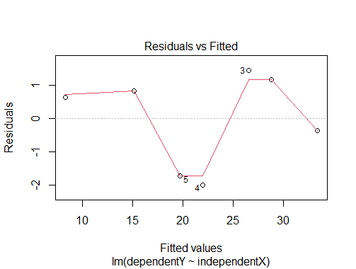
#in this we are performing the multi linear regression using the three independent #storing the three independent variables independentX1<-c(8,10,15,19,20,11,16,13,6,18)independentX2<-c(22,26,24,32,38,39,29,13,15,25)independentX3<-c(28,26,24,22,29,25,27,23,20,21)#storing the dependent variable ydependentY<-c(43,12,45,48,33,37,39,38,36,28)#performing the multilinear regression analysismultilinear<-lm(dependentY~independentX1+independentX2+independentX3)#printing the summary of the resultsummary(multilinear)plot(multilinear) |
Output:
Call:
lm(formula = dependentY ~ independentX1 + independentX2 + independentX3)

Residuals:
    Min      1Q  Median      3Q     Max
-21.862  -2.466   2.124   6.983  10.232

Coefficients:
              Estimate Std. Error t value Pr(>|t|)
(Intercept)   38.76188   35.43412   1.094    0.316
independentX1  0.46033    1.00476   0.458    0.663
independentX2 -0.09301    0.63260  -0.147    0.888
independentX3 -0.27250    1.55802  -0.175    0.867

Residual standard error: 12.22 on 6 degrees of freedom
Multiple R-squared:  0.04444,    Adjusted R-squared:  -0.4333
F-statistic: 0.093 on 3 and 6 DF,  p-value: 0.9612

Regression Analysis
Polynomial Regression
Polynomial regression analysis is a non linear regression analysis . Polynomial regression analysis helps for the flexible curve fitting of the data , involves the fitting of polynomial equation of the data.Polynomial regression analysis is the extension of the simple linear regression analysis by adding the extra independent variables obtained by raising the power .
The mathematical expression for the polynomail regression analysis is shown below.
y=a0+a1x+a2x^2+………..+anx^n
- where y is dependent variable
- x is independent variable
- a0,a1,a2 are the coefficeients of independent variable.
Let us now look at an example to fit a polynomial regression curve for the provided information.
|
x |
10 |
12 |
15 |
23 |
20 |
|
y |
14 |
7 |
23 |
25 |
21 |
Let us now fit a second degree polynomial curve for the above provided information. Inorder to fit the curve for the polynomial regression we need the normal equations for the second degree polynomial. We know the second degree polynomial can be represented as y=a0+a1x+a2x^2 .
In order to fit the regression for the above second degree equation we need to calculate the coeffiecient values a0,a1,a2 by using the normal equations.
Normal equations for the second degree polynomail is.
∑y = n*a0 + a1∑x + a2 ∑x^2
∑xy = a0∑x + a1∑x^2 + a2 ∑x^3
∑x^2y = a0∑x^2 + a1∑x^3 + a2 ∑x^4
where n is the total number of observations in the provided inforamtion
For the above given information the value of n is 5.
Let us now calculate the values of a0,a1 and a2.
|
x |
y |
x^2 |
x^3 |
x^4 |
xy |
x^2y |
|
10 |
14 |
100 |
1000 |
10000 |
140 |
1400 |
|
12 |
17 |
144 |
1728 |
20736 |
204 |
2448 |
|
15 |
23 |
225 |
3375 |
40500 |
345 |
5175 |
|
23 |
25 |
529 |
12167 |
279841 |
575 |
13225 |
|
20 |
21 |
400 |
8000 |
16000 |
420 |
8400 |
From the above table
- n=5 , ∑ x = 80 , ∑ y = 100 , ∑ x^2 = 1398 , ∑ x^3 = 26270 , ∑ x^4 = 521202 , ∑ xy = 1684 , ∑ x^2y = 30648
- Then the normal equations becomes :
- 100 = 5*a0 + 80*a1 + 1398*a2
- 1684 = 80*a0 + 1398*a1 + 26270*a2
- 30648 = 1398*a0 + 26270*a1 + 521202*a2
- By solving the above three equations we get a0 = -8.728 , a1 = 3.017 , a2 = -0.69
- The polynomial regression curve is y = -8.728 + 3.017x -0.69x^2 .
Now let us see the implementation of the polynomail regression in R .
R
#Storing the independent value XindependentX<-c(5,7,8,10,11,13,16)#soring the dependent valuedependentY<-c(33,30,28,20,18,16,9)#performing the regression analysis using the function lm with degree 3polyregression<-lm(dependentY~poly(independentX,degree=3))#printing the summary of the resultsummary(polyregression)#ploting the regression curveplot(polyregression) |
Output:
Call:
lm(formula = dependentY ~ poly(independentX, degree = 3))

Residuals:
      1       2       3       4       5       6       7
-0.4872  0.6943  1.1420 -1.6521 -1.0555  1.7218 -0.3632

Coefficients:
                                Estimate Std. Error t value Pr(>|t|)
(Intercept)                      22.0000     0.6533  33.673 5.76e-05 ***
poly(independentX, degree = 3)1 -20.8398     1.7286 -12.056  0.00123 **
poly(independentX, degree = 3)2   1.1339     1.7286   0.656  0.55866
poly(independentX, degree = 3)3   1.2054     1.7286   0.697  0.53578
---
Signif. codes:  0 ‘***’ 0.001 ‘**’ 0.01 ‘*’ 0.05 ‘.’ 0.1 ‘ ’ 1

Residual standard error: 1.729 on 3 degrees of freedom
Multiple R-squared:  0.9799,    Adjusted R-squared:  0.9598
F-statistic: 48.76 on 3 and 3 DF,  p-value: 0.004808

Regression Analysis
Exponential Regression
Expenential regression is a non linear type of regression . Exponential regression can be expressed in two ways . Let us discuss the both type of exponential regression types in detail with example . Exponential regression can be used in finance , biology , physics etc fields . Let us look the mathematical expression for the exponential regression with example.
y=ae^(bx)
- where y is dependent variable
- x is independent variable
- a , b are the regression coefficients.
While fitting the exponential curve , we can fit by converting the above equation in the form of line intercept form of straight line ( simple linear regression ) by applying the “ln” (logarithm with base e ) on both sides of the above equation y= ae^(bx).
By applying ln on both sides we get :
- ln(y) = ln(ae^(bx)) ->ln(y) = ln(a) + ln(e^(bx))
- ln(y) = ln(a) + bx
we can compare the above equation withe Y = A + BX
where Y=ln(y) , A = ln(a) , B=b , x=X , a=e^A and b=B
Normal equations will be
- ∑ Y = n*A + B ∑ X
- ∑ X*Y = A ∑ X + B ∑ X^2
Now let us try to fit an exponential regression for the given data
|
x |
1 |
5 |
7 |
9 |
12 |
|
y |
10 |
15 |
12 |
15 |
21 |
From the above derived equations we know X=x , Y=ln(y)
|
x |
y |
X |
Y = ln(y) |
X*Y |
X^2 |
|
1 |
10 |
1 |
2.302 |
2.302 |
1 |
|
5 |
15 |
5 |
2.708 |
13.54 |
25 |
|
7 |
12 |
7 |
2.484 |
17.388 |
49 |
|
9 |
15 |
9 |
2.708 |
24.372 |
81 |
|
12 |
21 |
12 |
3.044 |
36.528 |
144 |
From the above table n= 5 , ∑ X = 34 , ∑ Y = 13.246 ,∑ XY =94.13 , ∑ X^2 = 300
Now the normal equations becomes.
- 13.246 = 5A + 34B
- 94.13 = 34A + 300B
- By solving the above equation we can get the values of A and B
- A=2.248 and B= 0.059
- From the mentioned equations we know b=B and a=e^A
- a=e^2.248 =9.468
- b= B = 0.059
- The exponential regression equation is y=ae^(bx) -> y = 9.468*e^(0.059x)
Let us now try to implement the exponential regression in R programming
R
#storing the independent variableindependentX<-c(1,5,7,9,12)#storing the dependent variable dependentY<-c(10,15,12,15,21)#fitting the exponential regressionexponentialregression<-lm(log(dependentY,exp(1))~independentX)#determining the coefficients a and ba<-exp(coef(exponentialregression)[1])b<-coef(exponentialregression)[2]print(a)print(b)#printing the summary of exponential regression equationsummary(exponentialregression)#plotingplot(exponentialregression) |
Output:
(Intercept)
   66.54395

independentX
  -0.1185602


Call:
lm(formula = log(dependentY, exp(1)) ~ independentX)

Residuals:
        1         2         3         4         5         6         7
-0.108554  0.033256  0.082823 -0.016529 -0.003329  0.116008 -0.103675

Coefficients:
             Estimate Std. Error t value Pr(>|t|)
(Intercept)   4.19786    0.10862   38.65 2.19e-07 ***
independentX -0.11856    0.01026  -11.55 8.53e-05 ***
---
Signif. codes:  0 ‘***’ 0.001 ‘**’ 0.01 ‘*’ 0.05 ‘.’ 0.1 ‘ ’ 1

Residual standard error: 0.09406 on 5 degrees of freedom
Multiple R-squared:  0.9639,    Adjusted R-squared:  0.9567
F-statistic: 133.4 on 1 and 5 DF,  p-value: 8.527e-05

Regression Analysis
Exponential regression in the form of y=ab^x.
y=ab^x
where y is dependent variable
- x is independent variable
- a , b are the regression coefficients
While fitting the exponential curve , we can fit by converting the above equation in the form of line intercept form of straight line ( simple linear regression ) by applying the “log” (logarithm with base 10 ) on both sides of the above equation y= ab^x.
By applying ln on both sides we get :
- log10(y) = log10(ab^x) ->log10(y) = log10(a) + log10(b^x)
- log10(y) = log10(a) + xlog10(b)
we can compare the above equation withe Y = A + BX
where Y=log10(y) , A = log10(a) , B=log10(b) , x=X , a=10^A and b=10^B
Normal equations will be
- ∑ Y = n*A + B ∑ X
- ∑ X*Y = A ∑ X + B ∑ X^2
Now let us try to fit an exponential regression for the given data
|
x |
2 |
3 |
4 |
5 |
6 |
|
y |
8.3 |
15.4 |
33.1 |
165.2 |
127.4 |
From the above equation we know that X=x and Y=log10(y)
|
x |
y |
X |
X^2 |
Y=log10(y) |
XY |
|
2 |
8.3 |
2 |
4 |
0.91 |
1.82 |
|
3 |
15.4 |
3 |
9 |
1.18 |
3.54 |
|
4 |
33.1 |
4 |
16 |
1.51 |
6.04 |
|
5 |
165.2 |
5 |
25 |
2.21 |
11.05 |
|
6 |
127.4 |
6 |
36 |
2.1 |
12.6 |
From the above table n= 5 , ∑ X = 20 , ∑ Y = 7.91 ,∑ XY =35.05 , ∑ X^2 = 90
Now the normal equations becomes.
- 7.91 = 5A + 20B
- 35.05 = 20A + 90B
- By solving the above equation we can get the values of A and B
- A=0.218 and B= 0.341
- From the mentioned equations we know b=10^B and a=10^A
- a=10^0.218 = 1.6519
- b= 10^0.341 = 2.192
- The exponential regression equation is y=ab^x -> y = 1.6519*2.192^x
Let us now try to implement the exponential regression in R programming
R
#storing the independent variableindependentX<-c(2,3,4,5,6)#storing the dependent variable dependentY<-c(8.3,15.4,33.1,165.2,127.4)#fitting the exponential regressionexponentialregression<-lm(log10(dependentY)~independentX)#determining the coefficients a and ba<-10^(coef(exponentialregression)[1])b<-10^coef(exponentialregression)[2]print(a)print(b)#printing the summary of exponential regression equationsummary(exponentialregression)#plotingplot(exponentialregression) |
Output:
(Intercept)
   66.54395

independentX
   0.8881984

Call:
lm(formula = log10(dependentY) ~ independentX)

Residuals:
        1         2         3         4         5         6         7
-0.047144  0.014443  0.035970 -0.007178 -0.001446  0.050382 -0.045026

Coefficients:
              Estimate Std. Error t value Pr(>|t|)
(Intercept)   1.823109   0.047171   38.65 2.19e-07 ***
independentX -0.051490   0.004457  -11.55 8.53e-05 ***
---
Signif. codes:  0 ‘***’ 0.001 ‘**’ 0.01 ‘*’ 0.05 ‘.’ 0.1 ‘ ’ 1

Residual standard error: 0.04085 on 5 degrees of freedom
Multiple R-squared:  0.9639,    Adjusted R-squared:  0.9567
F-statistic: 133.4 on 1 and 5 DF,  p-value: 8.527e-05

Regression Analysis
Logistic Regression
Logistic regression analysis can be used for classification and regression .We can solve the logistic regression eqaution by using the linear regression representation. The mathematical equation of the logistic regression can be denoted in two ways as shown below.
y=a+b*ln(x)
where y is dependent variable
- x is independent variable
- β0 , β1 …. are the constants/regression coefficients
R
#logarthimic regression#storing dependent and independent variablesindependentX<-c(10,20,30,40,50,60,70,80,90)dependentY<-c(1,2,3,4,5,6,7,8,9)#fitting the logarithmic regression equationlogarthimic<-lm(dependentY~log(independentX,exp(1)))#printing the summary of resultsummary(logarthimic) |
Output:
Call:
lm(formula = dependentY ~ log(independentX, exp(1)))

Residuals:
      1       2       3       4       5       6       7
-2.4883  1.7209  2.5819 -0.6370 -0.5949  0.9843 -1.5668

Coefficients:
                          Estimate Std. Error t value Pr(>|t|)
(Intercept)                 69.972      4.710   14.86  2.5e-05 ***
log(independentX, exp(1))  -21.426      2.076  -10.32 0.000147 ***
---
Signif. codes:  0 ‘***’ 0.001 ‘**’ 0.01 ‘*’ 0.05 ‘.’ 0.1 ‘ ’ 1

Residual standard error: 2 on 5 degrees of freedom
Multiple R-squared:  0.9552,    Adjusted R-squared:  0.9462
F-statistic: 106.5 on 1 and 5 DF,  p-value: 0.000147
Steps in Regression Analysis
- Firstly , we need to identify the problem, objective or research question inorder to apply the regression analysis.
- Collect the required data or relevant data for the regression analysis. Make sure the data is free form errors and missed value.
- To understand the characteristics of the data perform EDA analysis which include data visualization , statistical summary of the data.
- We need to select the variables which are independent variables .
- After selection of the independent variables ,we need to perform the data preprocessing which includes the handling the missing data , outliers in the taken data.
- Then we need to build the model based on the type of the regression model we are performing.
- We need to estimate the parameters or coefficients of the regression model by using the estimation methods.
- After calculating the parameters , we need to check the model whether it is good fit for all the data or not . (i.e., checking the performance of the model).
- Finally use the model for unseen data .
Applications of regression analysis
Regression Analysis has various applications in many fields like economics,finance,real estate , healthcare , marketing ,business , science , education , psychology , sport analysis , agriculture and many more. Let us now discuss about the few applications of regression analysis .
- Regression analysis is used for the prediction of stock price based on the past data, analyzing the relationship between the interest rate and consumer spending.
- It can be used for the analysis of the impact of price changes on product demand and for predicting the sales based on expenditure of advertisement.
- It can be used in real estate for predicting the value of property based on the location.
- Regression is also used in the weather forecasting.
- It is also used for the prediction of crops yield based on the weather conditions , impact of fertilizers and irrigation the plant.
- It can be used in the analysis of the product quality and also gives the relationship between the manufacturing varibales and product quality.
- It can be used for the prediction of performance of the sports players based on the historical data and impact of coaching strategies on team sucess.
Advantages of regression analysis
- It provides insights how one or more independent variables relates to the dependent variables.
- It helps in analysis of the model and gives the relationship among the varibels.
- It helps in forecasting and decision making by predicting the dependent variables based on the independent variabels.
- Regression Analysis can help in predicting the most important predictor/variable among all other variables.
- It gives the information providing the strengths , positives and negatives of the relationship between the variables.
- The goodness of fit and identify potential issues of the model can be assessed by the diagnostic tools like residual analysis tools.
Disadvantages of regression analysis
- Regression Analysis is sentive to outliers which infulencing the coeffiecient estimation .
- Regression analysis dependents on the several assumptions like linearity , normality of residuals etc which effects the realibility of the results when the assumptions are violated.
- Regression Analysis mostly depend on the quality of the data . The results will be inaccurate and unrealiable when the data is biased .
- With the regression analysis we are not able to provide the accurate results for the extremely complex relationships.
- In regression analysis multi collinearity may lead to standard errors and it is becoming a challenge to identify the contribution of each variable in the data.
In this we have studied about the regression analysis , where it can be used , types of regression analysis , its applications in different fields , its advantages and disadvantages.
Reffered: https://www.geeksforgeeks.org
| AI ML DS |
Type: | Geek |
Category: | Coding |
Sub Category: | Tutorial |
Uploaded by: | Admin |
Views: | 12 |