Partial least square regression is a Machine learning Algorithm used for modelling the relationship between independent and dependent variables. This is mainly used when there are many interrelated independent variables. It is more commonly used in regression and latent variable modelling. It finds the directions (latent variables) in the independent variable space, explaining the maximum variance in both dependent and independent variables. It iteratively extracts the latent variables to find the maximum covariance between dependent and independent variables. The article explores more PLSRegression and implementation using the Sklearn library.

What is Partial Least Squares Regression?

Partial least squares regression (PLS regression) is a statistical technique that shares similarities with principal components regression. Instead of identifying hyperplanes of maximum variance between the response and independent variables, PLS regression constructs a linear regression model by projecting both the predicted and observable variables into a new space. This characteristic of projecting data to new spaces classifies PLS methods as bilinear factor models. Partial least squares discriminant analysis (PLS-DA) is a specific variant used when the response variable (Y) is categorical.

PLS is employed to uncover the underlying relationships between two matrices (X and Y). It takes a latent variable approach to model the covariance structures in these matrices. The objective of a PLS model is to identify a multidimensional direction in the X space that explains the maximum multidimensional variance direction in the Y space. PLS regression is particularly advantageous when the predictor matrix has more variables than observations and when there is multicollinearity among X values. This is in contrast to standard regression, which may struggle in these situations unless regularization is applied.

Partial Least Squares Regression Implementation

To implement PLS we are taking the “Diabetes” dataset. Now, let’s take a look at how PLS is used to predict diabetes progression. In this dataset, the “diabetes progression” variable is the dependent variable In the Diabetes dataset, independent variables would be the various health-related measurements such as age, sex, BMI, blood pressure, and other serum measurements. We use the PLS model to predict the “diabetes progression” (dependent variable) based on the “health-related measurements”(independent variables).

PLS algorithm iteratively extracts latent variables by adjusting weights to maximize the covariance between health-related measurements and diabetes progression. Once the PLS model is trained, you can use it to predict the diabetes progression for new observations based on their health-related measurements.

Install scikit learn if not already installed:

# Install sci-kit-learn if not already installed
!pip install scikit-learn

This will install the sci-kit-learn package which is used machine learning, it provides tools for data analysis and data modeling, including various machine learning algorithms, preprocessing techniques, and model evaluation tools.

Import Necessary Libraries:

We need to import some libraries which we will use in the next sections of the code, those are:

• NumPy Python: This library is used for numerical operations in python.
• matplotlib: This library is used for data visualization in python.
• from sklearn import datasets: This will import the ‘datasets’ module from sklearn which will give access to built-in datasets.
• from sklearn.cross_decomposition import PLSRegression: This will Import the PLSRegression class for performing PLS regression.
• from sklearn.model_selection import train_test_split: This will import the train_test_split function for splitting dataset int to training and testing.
• from sklearn.metrics import mean_squared_error: This will Imports the mean_squared_error function for calculating the Mean Squared Error.

Load the Diabetes dataset:

This will load the Diabetes dataset from sci-kit-learn. This dataset is commonly used for regression tasks. This dataset contains some attributes and target variables as follows:

Attributes:

• Age
• Sex
• BMI (Body Mass Index)
• BP (Average Blood Pressure)
• S1 (Total Serum Cholesterol)
• S2 (Low-Density Lipoproteins)
• S3 (High-Density Lipoproteins)
• S4 (Total Cholesterol / HDL Cholesterol ratio)
• S5 (log of serum triglycerides level)
• S6 (Blood sugar level)

Target Variable: A quantitative measure of disease progression one year after baseline.

The goal of our model is to predict the progression of diabetes based on these input features.

Extract features (X) and target variable (y):

Here, the X variable extracts the features (independent variables) from the dataset and the Y variable extracts the target variable (dependent variable) from the dataset.

Split the data into training and testing sets:

This will split the dataset into training and testing sets. we converted 80% of the dataset into a training set and 20% into a testing set and the random_state parameter ensures reproducibility.

Initialize the PLS model with the desired number of components:

Here we are given latent variables that should be 3 with the ‘n_components’ variable and initialized the PLS regression model with the specified number of components.

Fit the model on the training data:

Here it will train the PLS model using training data.

Predictions on the test set:

Here we used the PLS model to make predictions on test data

Evaluate the model performance:

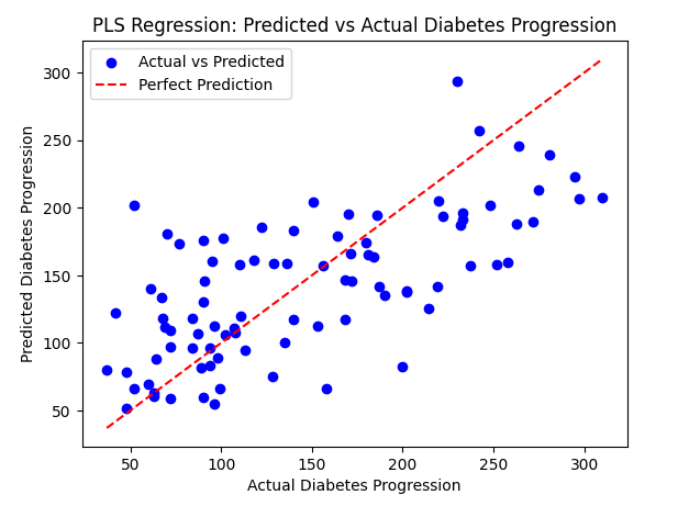
Output:

R-Squared Error: 0.46015344535176705
Mean Squared Error: 2860.1889674401987

Here, we calculated the Mean Squared Error between the actual and predicted values on the test set and printed the result.

Visualize predicted vs actual values:

Here, we used a scatter plot to compare the actual diabetes progression values to the predicted values. This visualization is useful for assessing the model’s performance.

Output:

PLS Regression: Predicted vs Actual Diabetes Progression

In this scatter plot, the blue points represent the actual versus predicted diabetes progression values for each data instance. The red dashed line represents a perfect prediction scenario where actual and predicted values are identical. Deviations from this line indicate the model’s predictive performance.

Using SHAP to interpret the PLS model:

SHAP (SHapley Additive explanations) is used for explaining the output of machine learning models by attributing the model’s prediction to each feature in a way that fairly distributes the contribution among the features.

Output: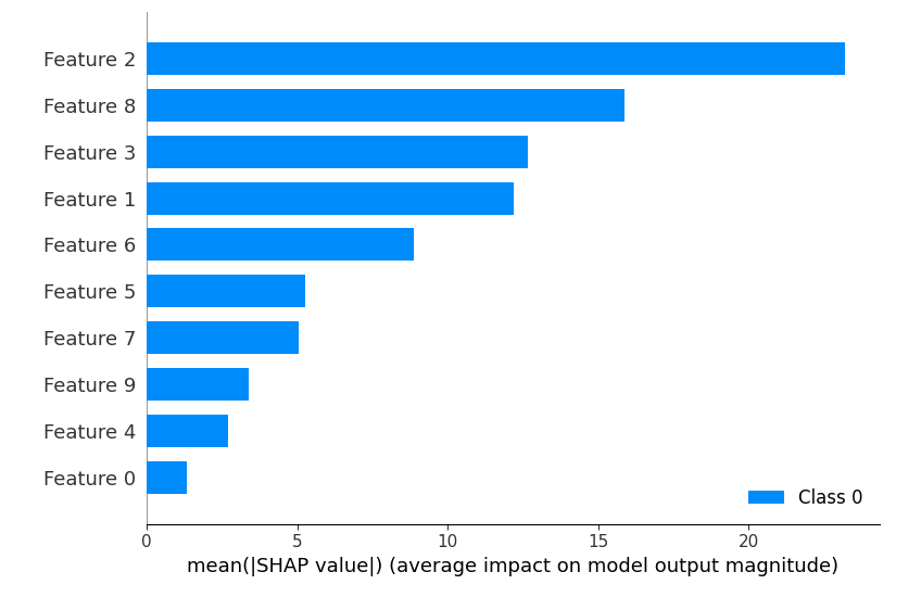

SHAP summary

Here, this plot provides a summary of the impact each feature has on the PLS model’s output across all instances in the test set. Positive and negative SHAP values indicate the direction and magnitude of the influence.

Google Colab Notebook

Why PLS is used?

• Multicollinearity: If there is high multicollinearity among the independent variables, then we can use PLS because it efficiently deals with when the predictors are highly correlated.
• High-Dimensional data: High-dimensional data means when the predictors are more than the number of observations. This Is common in fields like “Genomics” or “Spectroscopy”.
• Small Sample Size: If the number of observations is limited, PLS can provide stable results. It is less Prone to overfitting compared to traditional regression models.
• Simultaneous Modelling of Multiple Dependent Variables: PLS can be used to simulate predictions for multiple dependent variables. If there are multiple dependent and independent variables, then PLS allows for the simultaneous analysis of relationships between dependent and independent variables.
• Latent Variables Modelling: PLS, can be used for latent variable modeling. It is useful in some cases where the relations between variables are not directly observable.
• Predictive Performance: PLS is like having perfection for predictions, especially when a lot is going on with many predictors. It tends to do a better job of foreseeing outcomes compared to the usual prediction methods. Think of it as having a super-intuitive friend who’s surprisingly accurate at guessing what’s going to happen next.

Conclusion

In conclusion, Partial Least Squares (PLS) regression is a powerful and flexible statistical technique that finds widespread application in various fields. PLS is capable of handling multicollinearity, high-dimensional data, and complex relationships between predictor and response variables making it a valuable tool for researchers and practitioners. Despite its advantages, it’s important to be aware of potential disadvantages, such as the need for careful model tuning to avoid overfitting and its sensitivity to data preprocessing.