In machine learning, understanding decision boundaries is crucial for classification tasks. The decision boundary separates different classes in a dataset. Here, we’ll explore and compare decision boundaries generated by two popular classification algorithms – Label Propagation and Support Vector Machines (SVM) – using the famous Iris dataset in Python’s Scikit-Learn library.

Decision boundary of label Propagation vs SVM on the Iris dataset

On the Iris dataset, different decision boundaries are shown by Label Propagation and Support Vector Machines (SVM). Label propagation uses data point similarity to capture complex patterns. SVM, which aims for maximum margin, frequently draws distinct boundaries. The decision is based on the type of data and how complexity and interpretability are traded off.

It features 150 examples of three iris flower species: setosa, versicolor, and virginica. Each sample has four characteristics: sepal length, sepal width, petal length, and petal width. The idea is to use these traits to predict the species of a fresh sample.

There are several machine learning techniques available to handle this problem, including k-nearest neighbours, decision trees, logistic regression, and support vector machines (SVM). Some of these algorithms, however, demand that all of the samples have a known label, which may not be feasible in some cases. For instance, suppose we have a big dataset with just a few labelled examples and the others are unlabeled.

how can we use the information from the unlabeled samples to improve our predictions?

• One possible method is to utilize a semi-supervised learning technique, such as label propagation. Label propagation is a method that transfers labels from labeled samples to unlabeled samples based on their similarity. The distance, the kernel function, or the graph structure may all be used to determine similarity. The concept is that samples in the feature space that are near each other are likely to belong to the same class.
• In this post, we will evaluate the performance of label propagation and SVM on the Iris dataset, as well as visualize each algorithm’s decision boundary. To construct the algorithms and visualize the results, we will utilize Scikit Learn, a popular Python machine-learning framework.

Concepts of Decision boundary of label propagation vS SVM

Before we start coding, let us review some key concepts related to the topic:

Label Propagation

Label propagation is a semi-supervised learning algorithm that assigns labels to unlabeled samples based on the labels of their neighbors. The algorithm works as follows:

1. Initialize the label matrix Y with the known labels for the labeled samples, and -1 for the unlabeled samples.
2. Construct a weighted graph G, where each node represents a sample, and each edge represents the similarity between two samples. The similarity can be computed by various methods, such as the Euclidean distance, the Gaussian kernel, or the k-nearest neighbors graph.
3. Propagate the labels from the labeled nodes to the unlabeled nodes by updating the label matrix Y iteratively. The update rule is:
   
   where Yi is the i-th sample’s label, Wij is the weight of the edge between the i-th and j-th samples, and the total is over all samples. The update rule may be thought of as taking the weighted average of the neighbours’ labels.
4. Step 3 should be repeated until convergence is attained or a maximum number of iterations is reached.

The label propagation algorithm is a subset of the label spreading method that includes a regularization term in the update process to prevent overfitting. Scikit Learn includes the label spreading algorithm, which can be used instead of label propagation.

Support Vector Machines

• Support vector machines (SVM) are supervised learning algorithms that may be used to solve classification and regression issues. The main principle of SVM is to identify a hyperplane that separates samples of distinct classes with the greatest margin.
• A linear equation defines the hyperplane: wx+b=0
  • where w is the hyperplane’s normal vector, x is the sample’s feature vector, and b is the bias term. The samples on the margin are known as support vectors, and they define the ideal hyperplane.
• However, not all problems are linearly separable, which means that a hyperplane that can separate samples from different classes may not exist. In this case, we can use a kernel function to map the original feature space to a higher-dimensional space, where the problem may become linearly separable. A kernel function is one that computes the inner product of two vectors in the mapped space without performing the mapping explicitly. Some examples of common kernel functions are:
  
  
  
  

• The kernel function and its parameters can have an impact on the SVM algorithm’s performance. Scikit Learn provides several options for tuning the kernel function and other SVM algorithm hyperparameters.

Implementation of Decision boundary of label propagation vs SVM on the Iris dataset

Let’s understand the implementation of Decision boundary of label propagation versus SVM on the Iris dataset.

Import the necessary libraries and modules

Within our code, we’ll make use of the following modules and libraries:

• numpy: a library for scientific computing and linear algebra.
• matplotlib: a library for plotting and visualization.
• sklearn: a library for machine learning and data analysis.
• sklearn.datasets: a module that provides various datasets for machine learning.
• sklearn.semi_supervised: a module that provides semi-supervised learning algorithms, such as label propagation and label spreading.
• sklearn.svm: a module that provides support vector machines and related algorithms.
• sklearn.metrics: a module that provides various metrics for evaluating the performance of machine learning models.

Loading Dataset

The datasets module of scikit-learn is used in this Python code to load the Iris dataset. For the purpose of visualization or analysis, it extracts the first two features (X = iris.data[:, :2]) and their matching target labels (y = iris.target) using only these particular features.

Creating Mask for labeled and unlabeled samples

In order to designate a specific ratio (10%) of samples (n_labeled) as labeled and the remaining samples as unlabeled, this code creates a binary mask (mask). Next, using the generated mask, it makes a copy of the original target labels (y_unlabeled) and gives the unlabeled samples a value of -1. To ensure reproducibility, the random seed is fixed at 42.

Training and prediction of Model

Using the labeled samples, this code trains two models: Support Vector Machine (svm_model) and Label Propagation (lp_model). While SVM trains on labeled data using the fit method, Label Propagation uses the labeled samples to fit the model. Next, both models use the predict method to predict the labels of the unlabeled samples (X[~mask]); the predictions are then stored in y_pred_lp and y_pred_svm, respectively.

Evaluation of the model

Output:

Accuracy of label propagation: 0.76
Accuracy of SVM: 0.61

This code assesses the Label Propagation and SVM models’ accuracy using the unlabeled samples. The accuracy_score function from scikit-learn is utilized to compare the predicted labels (y_pred_lp and y_pred_svm) with the true labels (y[~mask]). The outcomes, which display each model’s accuracy on the unlabeled samples, are then printed.

Creating a Meshgrid

The range of the dataset’s first two features is covered by the meshgrid (xx and yy) defined by this code. After creating a grid of points using np.meshgrid, a matrix (mesh_input) representing points across the 2D feature space for contour plotting or decision boundary visualization is created by combining the flattened meshgrid coordinates (xx.ravel() and yy.ravel()) with np.c_.

Visualization of the Meshgrid

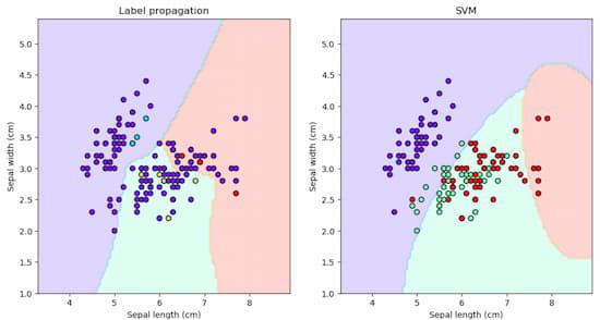
Output:

With the help of this code, decision boundaries for the Label Propagation and SVM models can be plotted side by side. It reshapes the results for contour plotting after predicting labels for the meshgrid points (mesh_input) in each subplot. Next, contourf is used to visualize the decision boundaries. Overlaid are scatter plots of labeled and unlabeled samples, with various colors denoting various classes. At last, the plot is displayed using the plt.show() command.

Conclusion

Using scikit-learn, several differences are seen between the decision boundaries of Label Propagation and SVM on the Iris dataset. Label propagation creates delicate decision boundaries that capture complex patterns by using similarity between data points. SVM, on the other hand, creates distinct, linear decision boundaries by aiming for the maximum margin. Based on the type of data and the balance between interpretability and complexity, one can choose between these models. For situations where simplicity and clarity are crucial, SVM offers clear-cut decision boundaries, whereas Label Propagation is excellent at capturing subtle relationships. The display highlights the different ways in which the models approached classification in this popular dataset.