This Asymptotic Analysis of Algorithms is a critical topic for the GATE (Graduate Aptitude Test in Engineering) exam, especially for candidates in computer science and related fields. This set of notes provides an in-depth understanding of how algorithms behave as input sizes grow and is fundamental for assessing their efficiency. Let’s delve into an introduction for these notes:

Introduction of Algorithms

The word Algorithm means “A set of rules to be followed in calculations or other problem-solving operations” Or “A procedure for solving a mathematical problem in a finite number of steps that frequently involves recursive operations “.

Therefore Algorithm refers to a sequence of finite steps to solve a particular problem. Algorithms can be simple and complex depending on what you want to achieve.

Types of Algorithms:

1. Brute Force Algorithm
2. Recursive Algorithm
3. Backtracking Algorithm
4. Searching Algorithm
5. Sorting Algorithm
6. Hashing Algorithm
7. Divide and Conquer Algorithm
8. Greedy Algorithm
9. Dynamic Programming Algorithm
10. Randomized Algorithm

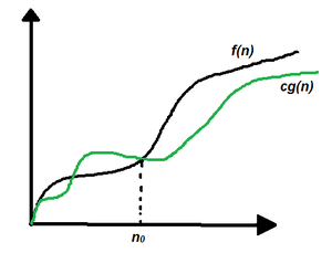
Asymptotic Notations

In mathematics, asymptotic analysis, also known as asymptotics, is a method of describing the limiting behavior of a function. In computing, asymptotic analysis of an algorithm refers to defining the mathematical boundation of its run-time performance based on the input size. For example, the running time of one operation is computed as f(n), and maybe for another operation, it is computed as g(n²). This means the first operation running time will increase linearly with the increase in n and the running time of the second operation will increase exponentially when n increases. Similarly, the running time of both operations will be nearly the same if n is small in value.

Usually, the analysis of an algorithm is done based on three cases:

1. Best Case (Omega Notation (Ω))
2. Average Case (Theta Notation (Θ))
3. Worst Case (O Notation(O))

Asymptotic Analysis

Given two algorithms for a task, how do we find out which one is better? 

One naive way of doing this is – to implement both the algorithms and run the two programs on your computer for different inputs and see which one takes less time. There are many problems with this approach for the analysis of algorithms. 

• It might be possible that for some inputs, the first algorithm performs better than the second. And for some inputs second performs better. 
• It might also be possible that for some inputs, the first algorithm performs better on one machine, and the second works better on another machine for some other inputs.

Asymptotic Analysis is the big idea that handles the above issues in analyzing algorithms. In Asymptotic Analysis, we evaluate the performance of an algorithm in terms of input size (we don’t measure the actual running time). We calculate, how the time (or space) taken by an algorithm increases with the input size. 

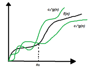
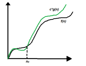
Measurement of Complexity of an Algorithm (Worst, Best and Average Case)

Based on the above three notations of Time Complexity there are three cases to analyze an algorithm:

1. Worst Case Analysis (Mostly used): Denoted by Big-O notation

In the worst-case analysis, we calculate the upper bound on the running time of an algorithm. We must know the case that causes a maximum number of operations to be executed. For Linear Search, the worst case happens when the element to be searched (x) is not present in the array. When x is not present, the search() function compares it with all the elements of arr[] one by one. Therefore, the worst-case time complexity of the linear search would be O(n).

2. Best Case Analysis (Very Rarely used): Denoted by Omega notation 

In the best-case analysis, we calculate the lower bound on the running time of an algorithm. We must know the case that causes a minimum number of operations to be executed. In the linear search problem, the best case occurs when x is present at the first location. The number of operations in the best case is constant (not dependent on n). So time complexity in the best case would be Ω(1) 

3. Average Case Analysis (Rarely used): Denoted by Theta notation 

In average case analysis, we take all possible inputs and calculate the computing time for all of the inputs. Sum all the calculated values and divide the sum by the total number of inputs. We must know (or predict) the distribution of cases. For the linear search problem, let us assume that all cases are uniformly distributed (including the case of x not being present in the array). So we sum all the cases and divide the sum by (n+1). Following is the value of average-case time complexity. 

How to Analyse Loops for Complexity Analysis of Algorithms?

Constant Time Complexity O(1):

The time complexity of a function (or set of statements) is considered as O(1) if it doesn’t contain a loop, recursion, and call to any other non-constant time function. 
 i.e. set of non-recursive and non-loop statements

In computer science, O(1) refers to constant time complexity, which means that the running time of an algorithm remains constant and does not depend on the size of the input. This means that the execution time of an O(1) algorithm will always take the same amount of time regardless of the input size. An example of an O(1) algorithm is accessing an element in an array using an index.

Linear Time Complexity O(n):

The Time Complexity of a loop is considered as O(n) if the loop variables are incremented/decremented by a constant amount. For example following functions have O(n) time complexity. Linear time complexity, denoted as O(n), is a measure of the growth of the running time of an algorithm proportional to the size of the input. In an O(n) algorithm, the running time increases linearly with the size of the input. For example, searching for an element in an unsorted array or iterating through an array and performing a constant amount of work for each element would be O(n) operations. In simple words, for an input of size n, the algorithm takes n steps to complete the operation.

Quadratic Time Complexity O(n^c):

The time complexity is defined as an algorithm whose performance is directly proportional to the squared size of the input data, as in nested loops it is equal to the number of times the innermost statement is executed. For example, the following sample loops have O(n²) time complexity 

Quadratic time complexity, denoted as O(n^2), refers to an algorithm whose running time increases proportional to the square of the size of the input. In other words, for an input of size n, the algorithm takes n * n steps to complete the operation. An example of an O(n^2) algorithm is a nested loop that iterates over the entire input for each element, performing a constant amount of work for each iteration. This results in a total of n * n iterations, making the running time quadratic in the size of the input.

Logarithmic Time Complexity O(Log n):

The time Complexity of a loop is considered as O(Logn) if the loop variables are divided/multiplied by a constant amount. And also for recursive calls in the recursive function, the Time Complexity is considered as O(Logn).

Logarithmic Time Complexity O(Log Log n):

The Time Complexity of a loop is considered as O(LogLogn) if the loop variables are reduced/increased exponentially by a constant amount. 

How to combine the time complexities of consecutive loops? 

When there are consecutive loops, we calculate time complexity as a sum of the time complexities of individual loops. 

To combine the time complexities of consecutive loops, you need to consider the number of iterations performed by each loop and the amount of work performed in each iteration. The total time complexity of the algorithm can be calculated by multiplying the number of iterations of each loop by the time complexity of each iteration and taking the maximum of all possible combinations.

For example, consider the following code:

for i in range(n):
for j in range(m):
# some constant time operation

Here, the outer loop performs n iterations, and the inner loop performs m iterations for each iteration of the outer loop. So, the total number of iterations performed by the inner loop is n * m, and the total time complexity is O(n * m).

In another example, consider the following code:

for i in range(n):
for j in range(i):
# some constant time operation

Here, the outer loop performs n iterations, and the inner loop performs i iterations for each iteration of the outer loop, where i is the current iteration count of the outer loop. The total number of iterations performed by the inner loop can be calculated by summing the number of iterations performed in each iteration of the outer loop, which is given by the formula sum(i) from i=1 to n, which is equal to n * (n + 1) / 2. Hence, the total time complex

Algorithms Cheat Sheet for Complexity Analysis:

Runtime Analysis of Algorithms:

In general cases, we mainly used to measure and compare the worst-case theoretical running time complexities of algorithms for the performance analysis. 
The fastest possible running time for any algorithm is O(1), commonly referred to as Constant Running Time. In this case, the algorithm always takes the same amount of time to execute, regardless of the input size. This is the ideal runtime for an algorithm, but it’s rarely achievable. 
In actual cases, the performance (Runtime) of an algorithm depends on n, that is the size of the input or the number of operations is required for each input item. 
The algorithms can be classified as follows from the best-to-worst performance (Running Time Complexity): 

•  A logarithmic algorithm – O(logn) 
  Runtime grows logarithmically in proportion to n. 
•  A linear algorithm – O(n) 
  Runtime grows directly in proportion to n. 
•  A superlinear algorithm – O(nlogn) 
  Runtime grows in proportion to n. 
•  A polynomial algorithm – O(n^c) 
  Runtime grows quicker than previous all based on n. 
•  A exponential algorithm – O(cⁿ) 
  Runtime grows even faster than polynomial algorithm based on n. 
•  A factorial algorithm – O(n!) 
  Runtime grows the fastest and becomes quickly unusable for even 
  small values of n.  

Little o and Little omega notations:

Little-o: Big-O is used as a tight upper bound on the growth of an algorithm’s effort (this effort is described by the function f(n)), even though, as written, it can also be a loose upper bound. “Little-o” (o()) notation is used to describe an upper bound that cannot be tight. 

Definition: Let f(n) and g(n) be functions that map positive integers to positive real numbers. We say that f(n) is o(g(n)) if for any real constant c > 0, there exists an integer constant n0 > 1 such that 0 < f(n) < c*g(n).

 Thus, little o() means loose upper-bound of f(n). Little o is a rough estimate of the maximum order of growth whereas Big-O may be the actual order of growth.  

little-omega:

The relationship between Big Omega (Ω) and Little Omega (ω) is similar to that of Big-O and Little o except that now we are looking at the lower bounds. Little Omega (ω) is a rough estimate of the order of the growth whereas Big Omega (Ω) may represent exact order of growth. We use ω notation to denote a lower bound that is not asymptotically tight.

Definition : Let f(n) and g(n) be functions that map positive integers to positive real numbers. We say that f(n) is ω(g(n)) if for any real constant c > 0, there exists an integer constant n0 > 1 such that f(n) > c * g(n) > 0 for every integer n > n0. 

f(n) has a higher growth rate than g(n) so main difference between Big Omega (Ω) and little omega (ω) lies in their definitions.In the case of Big Omega f(n)=Ω(g(n)) and the bound is 0<=cg(n)<=f(n), but in case of little omega, it is true for 0<=c*g(n)<f(n).

What does ‘Space Complexity’ mean?

The term Space Complexity is misused for Auxiliary Space at many places. Following are the correct definitions of Auxiliary Space and Space Complexity. 

Auxiliary Space is the extra space or temporary space used by an algorithm. The space Complexity of an algorithm is the total space taken by the algorithm with respect to the input size. Space complexity includes both Auxiliary space and space used by input. 

For example, if we want to compare standard sorting algorithms on the basis of space, then Auxiliary Space would be a better criterion than Space Complexity. Merge Sort uses O(n) auxiliary space, Insertion sort, and Heap Sort use O(1) auxiliary space. The space complexity of all these sorting algorithms is O(n) though. 

Space complexity is a parallel concept to time complexity. If we need to create an array of size n, this will require O(n) space. If we create a two-dimensional array of size n*n, this will require O(n²) space.

In recursive calls stack space also counts. 

Example : 

int add (int n){
if (n <= 0){
return 0;
}
return n + add (n-1);
}

Here each call add a level to the stack :

1. add(4)
2. -> add(3)
3. -> add(2)
4. -> add(1)
5. -> add(0)
Each of these calls is added to call stack and takes up actual memory.
So it takes O(n) space.

However, just because you have n calls total doesn’t mean it takes O(n) space.
Look at the below function :

int addSequence (int n){
int sum = 0;
for (int i = 0; i < n; i++){
sum += pairSum(i, i+1);
}
return sum;
}
int pairSum(int x, int y){
return x + y;
}

There will be roughly O(n) calls to pairSum. However, those
calls do not exist simultaneously on the call stack,
so you only need O(1) space.

Previous Year GATE Questions:

1. What is the worst-case time complexity of inserting n elements into an empty linked list, if the linked list needs to be maintained in sorted order? More than one answer may be correct. [GATE CSE 2020]

(A) Θ(n)

(B) Θ(n log n)

(C) Θ(n²)

(D) Θ(1)

Solution: Correct answer is (C)

2. What is the worst-case time complexity of inserting n² elements into an AVL tree with n elements initially? [GATE CSE 2020]

(A) Θ(n⁴)

(B) Θ(n²)

(C) Θ(n² log n)

(D) Θ(n³)

Solution: Correct answer is (C)

3. Which of the given options provides the increasing order of asymptotic complexity of functions f1, f2, f3 and f4? [GATE CSE 2011]
f1(n) = 2^n
f2(n) = n^(3/2)
f3(n) = nLogn
f4(n) = n^(Logn)

(A) f3, f2, f4, f1
(B) f3, f2, f1, f4
(C) f2, f3, f1, f4
(D) f2, f3, f4, f1

Answer: (A)
Explanation: nLogn is the slowest growing function, then comes n^(3/2), then n^(Logn).  Finally, 2^n is the fastest growing function.

4. Which one of the following statements is TRUE for all positive functions f(n)? [GATE CSE 2022]

(A) f(n²) = θ(f(n)²), when f(n) is a polynomial
(B) f(n²) = o(f(n)²)
(C) f(n²) = O(f(n)²), when f(n) is an exponential function
(D) f(n²) = Ω(f(n)²)

Solution: Correct answer is (A)

5.The tightest lower bound on the number of comparisons, in the worst case, for comparison-based sorting is of the order of [GATE CSE 2004]

(A) n
(B) n²
(C) n log n
(D) n log² n

Solution: Correct answer is (C)

6. Consider the following functions from positives integers to real numbers

10, √n, n, log₂n, 100/n.

The CORRECT arrangement of the above functions in increasing order of asymptotic complexity is:
(A) log₂n, 100/n, 10, √n, n
(B) 100/n, 10, log₂n, √n, n
(C) 10, 100/n ,√n, log₂n, n
(D) 100/n, log₂n, 10 ,√n, n

Answer: (B)

Explanation: For the large number, value of inverse of number is less than a constant and value of constant is less than value of square root.

10 is constant, not affected by value of n.
√n Square root and log₂n is logarithmic. So log₂n is definitely less than √n
n has linear growth and 100/n grows inversely with value of n. For bigger value of n, we can consider it 0, so 100/n is least and n is max.

7. Consider the following three claims

1. (n + k)^m = Θ(n^m), where k and m are constants

2. 2^{n + 1} = O(2ⁿ)

3. 2^{2n + 1} = O(2ⁿ)

Which of these claims are correct ?

(A) 1 and 2
(B) 1 and 3
(C) 2 and 3
(D) 1, 2, and 3

Answer: (A)

Explanation: (n + k)^m and Θ(n^m) are asymptotically same as theta notation can always be written by taking the leading order term in a polynomial expression.

2^{n + 1} and O(2ⁿ) are also asymptotically same as 2^{n + 1} can be written as 2 * 2ⁿ and constant multiplication/addition doesn’t matter in theta notation.

2^{2n + 1} and O(2ⁿ) are not same as constant is in power.

8. Consider the following three functions.

f1 = 10ⁿ
f2 = n^logn
f3 = n^√n

Which one of the following options arranges the functions in the increasing order of asymptotic growth rate?
(A) f3,f2,f1
(B) f2,f1,f3
(C) f1,f2,f3
(D) f2,f3,f1

Answer: (D)

Explanation: On comparing power of these given functions :
f1 has n in power.
f2 has logn in power.
f3 has √n in power.

Hence, f2, f3, f1 is in increasing order.

Note that you can take the log of each function then compare.