|
|
When dealing with classification problems that involve multiple classes or outcomes, it’s essential to have a reliable method for making predictions. One popular algorithm for such tasks is k-Nearest Neighbors (k-NN). In this tutorial, we will walk you through the process of making predictions with multiple outcomes using a k-NN model in R, specifically with the tidymodels framework. K-Nearest Neighbors (KNN) is a simple yet effective supervised machine learning algorithm used for classification and regression tasks. Here’s an explanation of KNN and some of its benefits: K-Nearest Neighbors (KNN):KNN is a non-parametric algorithm, meaning it doesn’t make any underlying assumptions about the distribution of data. It’s an instance-based or memory-based learning algorithm, which means it memorizes the entire training dataset and uses it to make predictions. The fundamental idea behind KNN is to classify a new data point by considering the majority class among its K-nearest neighbors. How KNN Works:
Benefits of KNN:
However, KNN also has some limitations. It can be computationally expensive for large datasets, and the choice of the distance metric and K value can significantly impact its performance. Additionally, it doesn’t provide insights into feature importance, which can be essential in some applications. TidymodelsTidymodels is a powerful and user-friendly ecosystem for modeling and machine learning in R. It provides a structured workflow for creating, tuning, and evaluating models. Before we proceed, make sure you have tidymodels and the necessary packages installed. You can install them using: R
Now, let’s dive into the steps to get predictions with multiple outcomes using a k-NN model. Pre-RequisitesBefore moving forward make sure you have Caret and ggplot packages installed. R
Load Required Libraries and DataWe’ll start by loading the necessary libraries and a dataset. For this tutorial, we’ll use the classic Iris dataset, which contains three different species of iris flowers (setosa, versicolor, and virginica). R
Preprocess DataData preprocessing is crucial for building a robust model. In this step, we’ll create a recipe to preprocess the data. In our case, we don’t need any preprocessing since the Iris dataset is well-structured and doesn’t have any missing values. R
Create and Train the k-NN ModelNow, it’s time to create and train our k-NN model. We’ll use the `nearest_neighbor()` function from the `parsnip` package, which is part of tidymodels. R
Output: + Fold1: kmax= 5, distance=2, kernel=optimal
- Fold1: kmax= 5, distance=2, kernel=optimal
+ Fold1: kmax= 7, distance=2, kernel=optimal
- Fold1: kmax= 7, distance=2, kernel=optimal
+ Fold1: kmax= 9, distance=2, kernel=optimal
- Fold1: kmax= 9, distance=2, kernel=optimal
+ Fold1: kmax=11, distance=2, kernel=optimal
- Fold1: kmax=11, distance=2, kernel=optimal
+ Fold1: kmax=13, distance=2, kernel=optimal
- Fold1: kmax=13, distance=2, kernel=optimal
+ Fold2: kmax= 5, distance=2, kernel=optimal
- Fold2: kmax= 5, distance=2, kernel=optimal
+ Fold2: kmax= 7, distance=2, kernel=optimal
- Fold2: kmax= 7, distance=2, kernel=optimal
+ Fold2: kmax= 9, distance=2, kernel=optimal
- Fold2: kmax= 9, distance=2, kernel=optimal
+ Fold2: kmax=11, distance=2, kernel=optimal
- Fold2: kmax=11, distance=2, kernel=optimal
+ Fold2: kmax=13, distance=2, kernel=optimal
- Fold2: kmax=13, distance=2, kernel=optimal
+ Fold3: kmax= 5, distance=2, kernel=optimal
- Fold3: kmax= 5, distance=2, kernel=optimal
+ Fold3: kmax= 7, distance=2, kernel=optimal
- Fold3: kmax= 7, distance=2, kernel=optimal
+ Fold3: kmax= 9, distance=2, kernel=optimal
- Fold3: kmax= 9, distance=2, kernel=optimal
+ Fold3: kmax=11, distance=2, kernel=optimal
- Fold3: kmax=11, distance=2, kernel=optimal
+ Fold3: kmax=13, distance=2, kernel=optimal
- Fold3: kmax=13, distance=2, kernel=optimal
+ Fold4: kmax= 5, distance=2, kernel=optimal
- Fold4: kmax= 5, distance=2, kernel=optimal
+ Fold4: kmax= 7, distance=2, kernel=optimal
- Fold4: kmax= 7, distance=2, kernel=optimal
+ Fold4: kmax= 9, distance=2, kernel=optimal
- Fold4: kmax= 9, distance=2, kernel=optimal
+ Fold4: kmax=11, distance=2, kernel=optimal
- Fold4: kmax=11, distance=2, kernel=optimal
+ Fold4: kmax=13, distance=2, kernel=optimal
- Fold4: kmax=13, distance=2, kernel=optimal
+ Fold5: kmax= 5, distance=2, kernel=optimal
- Fold5: kmax= 5, distance=2, kernel=optimal
+ Fold5: kmax= 7, distance=2, kernel=optimal
- Fold5: kmax= 7, distance=2, kernel=optimal
+ Fold5: kmax= 9, distance=2, kernel=optimal
- Fold5: kmax= 9, distance=2, kernel=optimal
+ Fold5: kmax=11, distance=2, kernel=optimal
- Fold5: kmax=11, distance=2, kernel=optimal
+ Fold5: kmax=13, distance=2, kernel=optimal
- Fold5: kmax=13, distance=2, kernel=optimal
Aggregating results
Selecting tuning parameters
Fitting kmax = 9, distance = 2, kernel = optimal on full training set
R
Output: k-Nearest Neighbors
This code sets up a k-NN classification model using the “kknn” method, performs cross-validation with different values of `k`, and prints information about the model specification. It’s a common practice in machine learning to explore different hyperparameters (like `k` in k-NN) to find the best model for a given problem. The resulting `knn_fit` will contain the trained and tuned k-NN model. Make PredictionsWith our trained k-NN model, we can now make predictions. We’ll use the `predict()` function to predict the species of iris flowers. R
Output: [1] setosa setosa setosa setosa setosa setosa
[7] setosa setosa setosa setosa setosa setosa
[13] setosa setosa setosa setosa setosa setosa
[19] setosa setosa setosa setosa setosa setosa
[25] setosa setosa setosa setosa setosa setosa
[31] setosa setosa setosa setosa setosa setosa
[37] setosa setosa setosa setosa setosa setosa
[43] setosa setosa setosa setosa setosa setosa
[49] setosa setosa versicolor versicolor versicolor versicolor
[55] versicolor versicolor versicolor versicolor versicolor versicolor
[61] versicolor versicolor versicolor versicolor versicolor versicolor
[67] versicolor versicolor versicolor versicolor versicolor versicolor
[73] versicolor versicolor versicolor versicolor versicolor versicolor
[79] versicolor versicolor versicolor versicolor versicolor versicolor
[85] versicolor versicolor versicolor versicolor versicolor versicolor
[91] versicolor versicolor versicolor versicolor versicolor versicolor
[97] versicolor versicolor versicolor versicolor virginica virginica
[103] virginica virginica virginica virginica versicolor virginica
[109] virginica virginica virginica virginica virginica virginica
[115] virginica virginica virginica virginica virginica versicolor
[121] virginica virginica virginica virginica virginica virginica
[127] virginica virginica virginica virginica virginica virginica
[133] virginica virginica virginica virginica virginica virginica
[139] virginica virginica virginica virginica virginica virginica
[145] virginica virginica virginica virginica virginica virginica
Levels: setosa versicolor virginica
The `predictions` object now contains the predicted species for each observation in the dataset. Evaluate the Model (Optional)Optionally, you can evaluate the performance of your model using various metrics like accuracy, precision, recall, or F1-score. The tidymodels framework provides functions for model evaluation, making it easy to assess your model’s performance. R
Output: Confusion Matrix and Statistics
Reference
Prediction setosa versicolor virginica
setosa 50 0 0
versicolor 0 50 2
virginica 0 0 48
Overall Statistics
Accuracy : 0.9867
95% CI : (0.9527, 0.9984)
No Information Rate : 0.3333
P-Value [Acc > NIR] : < 2.2e-16
Kappa : 0.98
Mcnemar's Test P-Value : NA
Statistics by Class:
Class: setosa Class: versicolor Class: virginica
Sensitivity 1.0000 1.0000 0.9600
Specificity 1.0000 0.9800 1.0000
Pos Pred Value 1.0000 0.9615 1.0000
Neg Pred Value 1.0000 1.0000 0.9804
Prevalence 0.3333 0.3333 0.3333
Detection Rate 0.3333 0.3333 0.3200
Detection Prevalence 0.3333 0.3467 0.3200
Balanced Accuracy 1.0000 0.9900 0.9800
Accuracy
0.9866667
[1] NA
[1] NA
In summary, the output provides a comprehensive assessment of the model’s classification performance, including accuracy, precision, recall, and other related statistics for each class in the dataset. The model appears to perform very well, with high accuracy and good class-specific metrics. Performing KNN on MTCars DatasetPerforming simple EDA on the “mtcars” dataset, using head and summary functions:R
Output: mpg cyl disp hp drat wt qsec vs am gear carb
Mazda RX4 21.0 6 160.0 110 3.90 2.620 16.46 0 1 4 4
Mazda RX4 Wag 21.0 6 160.0 110 3.90 2.875 17.02 0 1 4 4
Datsun 710 22.8 4 108.0 93 3.85 2.320 18.61 1 1 4 1
Hornet 4 Drive 21.4 6 258.0 110 3.08 3.215 19.44 1 0 3 1
Hornet Sportabout 18.7 8 360.0 175 3.15 3.440 17.02 0 0 3 2
Valiant 18.1 6 225.0 105 2.76 3.460 20.22 1 0 3 1
Duster 360 14.3 8 360.0 245 3.21 3.570 15.84 0 0 3 4
Merc 240D 24.4 4 146.7 62 3.69 3.190 20.00 1 0 4 2
Merc 230 22.8 4 140.8 95 3.92 3.150 22.90 1 0 4 2
Merc 280 19.2 6 167.6 123 3.92 3.440 18.30 1 0 4 4
Merc 280C 17.8 6 167.6 123 3.92 3.440 18.90 1 0 4 4
Merc 450SE 16.4 8 275.8 180 3.07 4.070 17.40 0 0 3 3
Merc 450SL 17.3 8 275.8 180 3.07 3.730 17.60 0 0 3 3
Merc 450SLC 15.2 8 275.8 180 3.07 3.780 18.00 0 0 3 3
Cadillac Fleetwood 10.4 8 472.0 205 2.93 5.250 17.98 0 0 3 4
Lincoln Continental 10.4 8 460.0 215 3.00 5.424 17.82 0 0 3 4
Chrysler Imperial 14.7 8 440.0 230 3.23 5.345 17.42 0 0 3 4
Fiat 128 32.4 4 78.7 66 4.08 2.200 19.47 1 1 4 1
Honda Civic 30.4 4 75.7 52 4.93 1.615 18.52 1 1 4 2
Toyota Corolla 33.9 4 71.1 65 4.22 1.835 19.90 1 1 4 1
Toyota Corona 21.5 4 120.1 97 3.70 2.465 20.01 1 0 3 1
Dodge Challenger 15.5 8 318.0 150 2.76 3.520 16.87 0 0 3 2
AMC Javelin 15.2 8 304.0 150 3.15 3.435 17.30 0 0 3 2
Camaro Z28 13.3 8 350.0 245 3.73 3.840 15.41 0 0 3 4
Pontiac Firebird 19.2 8 400.0 175 3.08 3.845 17.05 0 0 3 2
Fiat X1-9 27.3 4 79.0 66 4.08 1.935 18.90 1 1 4 1
Porsche 914-2 26.0 4 120.3 91 4.43 2.140 16.70 0 1 5 2
Lotus Europa 30.4 4 95.1 113 3.77 1.513 16.90 1 1 5 2
Ford Pantera L 15.8 8 351.0 264 4.22 3.170 14.50 0 1 5 4
Ferrari Dino 19.7 6 145.0 175 3.62 2.770 15.50 0 1 5 6
Maserati Bora 15.0 8 301.0 335 3.54 3.570 14.60 0 1 5 8
Volvo 142E 21.4 4 121.0 109 4.11 2.780 18.60 1 1 4 2
Summary of the DatasetR
Output: mpg cyl disp hp
Min. :10.40 Min. :4.000 Min. : 71.1 Min. : 52.0
1st Qu.:15.43 1st Qu.:4.000 1st Qu.:120.8 1st Qu.: 96.5
Median :19.20 Median :6.000 Median :196.3 Median :123.0
Mean :20.09 Mean :6.188 Mean :230.7 Mean :146.7
3rd Qu.:22.80 3rd Qu.:8.000 3rd Qu.:326.0 3rd Qu.:180.0
Max. :33.90 Max. :8.000 Max. :472.0 Max. :335.0
drat wt qsec vs
Min. :2.760 Min. :1.513 Min. :14.50 Min. :0.0000
1st Qu.:3.080 1st Qu.:2.581 1st Qu.:16.89 1st Qu.:0.0000
Median :3.695 Median :3.325 Median :17.71 Median :0.0000
Mean :3.597 Mean :3.217 Mean :17.85 Mean :0.4375
3rd Qu.:3.920 3rd Qu.:3.610 3rd Qu.:18.90 3rd Qu.:1.0000
Max. :4.930 Max. :5.424 Max. :22.90 Max. :1.0000
am gear carb
Min. :0.0000 Min. :3.000 Min. :1.000
1st Qu.:0.0000 1st Qu.:3.000 1st Qu.:2.000
Median :0.0000 Median :4.000 Median :2.000
Mean :0.4062 Mean :3.688 Mean :2.812
3rd Qu.:1.0000 3rd Qu.:4.000 3rd Qu.:4.000
Max. :1.0000 Max. :5.000 Max. :8.000
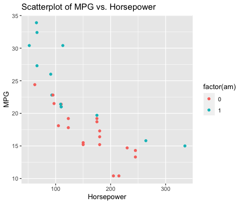
Creating visualizations to interpret the datasetR
Output:
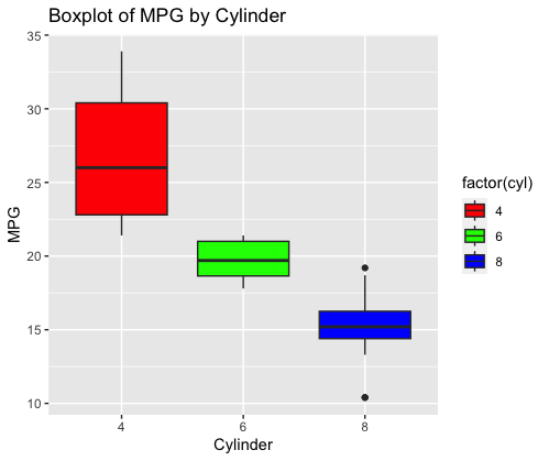
R
Output:
Creating the KNN modelR
Output: + Fold1: k= 5
- Fold1: k= 5
+ Fold1: k= 7
- Fold1: k= 7
+ Fold1: k= 9
- Fold1: k= 9
+ Fold1: k=11
- Fold1: k=11
+ Fold1: k=13
- Fold1: k=13
+ Fold2: k= 5
- Fold2: k= 5
+ Fold2: k= 7
- Fold2: k= 7
+ Fold2: k= 9
- Fold2: k= 9
+ Fold2: k=11
- Fold2: k=11
+ Fold2: k=13
- Fold2: k=13
+ Fold3: k= 5
- Fold3: k= 5
+ Fold3: k= 7
- Fold3: k= 7
+ Fold3: k= 9
- Fold3: k= 9
+ Fold3: k=11
- Fold3: k=11
+ Fold3: k=13
- Fold3: k=13
+ Fold4: k= 5
- Fold4: k= 5
+ Fold4: k= 7
- Fold4: k= 7
+ Fold4: k= 9
- Fold4: k= 9
+ Fold4: k=11
- Fold4: k=11
+ Fold4: k=13
- Fold4: k=13
+ Fold5: k= 5
- Fold5: k= 5
+ Fold5: k= 7
- Fold5: k= 7
+ Fold5: k= 9
- Fold5: k= 9
+ Fold5: k=11
- Fold5: k=11
+ Fold5: k=13
- Fold5: k=13
Aggregating results
Selecting tuning parameters
Fitting k = 5 on full training set
R
Output: k-Nearest Neighbors
32 samples
10 predictors
No pre-processing
Resampling: Cross-Validated (5 fold)
Summary of sample sizes: 26, 25, 26, 26, 25
Resampling results across tuning parameters:
k RMSE Rsquared MAE
5 0.4292704 0.4401123 0.3019048
7 0.4089749 0.5099996 0.3054422
9 0.4203775 0.5427578 0.3333333
11 0.4267676 0.5400401 0.3501443
13 0.4357731 0.5447669 0.3782051
RMSE was used to select the optimal model using the smallest value.
The final value used for the model was k = 7.
The code performs the following steps:
ConclusionIn this tutorial, we’ve shown you how to make predictions with multiple outcomes using a k-NN model in tidymodels. The key steps involve loading data, preprocessing it, creating and training the model, making predictions, and optionally evaluating the model’s performance. Tidymodels simplifies the entire process, allowing you to focus on building and assessing models rather than dealing with low-level details. It’s a valuable tool for anyone working on classification tasks with multiple outcomes. |
Reffered: https://www.geeksforgeeks.org
| R Language |
Type: | Geek |
Category: | Coding |
Sub Category: | Tutorial |
Uploaded by: | Admin |
Views: | 13 |