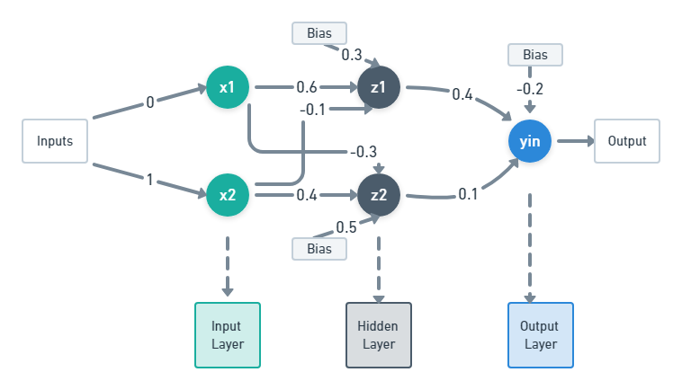
Let’s understand how errors are calculated and weights are updated in backpropagation networks(BPNs).

Consider the following network in the below figure.

Backpropagation Network (BPN)

The network in the above figure is a simple multi-layer feed-forward network or backpropagation network. It contains three layers, the input layer with two neurons x₁ and x₂, the hidden layer with two neurons z₁ and z₂ and the output layer with one neuron y_in. 

Now let’s write down the weights and bias vectors for each neuron. 

Note: The weights are taken randomly.

Input layer: i/p – [x₁ x₂] = [0 1]

Here since it is the input layer only the input values are present.

Hidden layer: z₁ – [v₁₁ v₂₁ v₀₁] = [0.6 -0.1 03]

Here v₁₁ refers to the weight of first input x₁ on z₁, v₂₁ refers to the weight of second input x₂ on z₁ and v₀₁ refers to the bias value on z₁.

z₂ – [v₁₂ v₂₂ v₀₂] = [-0.3 0.4 0.5]

Here v₁₂ refers to the weight of first input x₁ on z₂, v₂₂ refers to the weight of second input x₂ on z₂ and v₀₂ refers to the bias value on z₂.

Output layer: y_in – [w₁₁ w₂₁ w₀₁] = [0.4 0.1 -0.2]

Here w₁₁ refers to the weight of first neuron z₁ in a hidden layer on y_in, w₂₁ refers to the weight of second neuron z₂ in a hidden layer on y_in and w₀₁ refers to the bias value on y_in. Let’s consider three variables, k which refers to the neurons in the output layer, ‘j’ which refers to the neurons in the hidden layer and ‘i’ which refers to the neurons in the input layer.

Therefore, 

k = 1

j = 1, 2(meaning first neuron and second neuron in hidden layer)

i = 1, 2(meaning first and second neuron in the input layer)

Below are some conditions to be followed in BPNs.

Conditions/Constraints:

1. In BPN, the activation function used should be differentiable.
2. The input for bias is always 1.

To proceed with the problem, let:

Target value, t = 1

Learning rate, α = 0.25

Activation function = Binary sigmoid function

Binary sigmoid function, f(x) = (1+e^-x)^-1       eq. (1)

And, f'(x) = f(x)[1-f(x)]       eq. (2)

There are three steps to solve the problem:

1. Computing the output, y.
2. Backpropagation of errors, i.e., between output and hidden layer, hidden and input layer.
3. Updating weights.

Step 1:

The value y is calculated by finding y_in and applying the activation function.

y_in is calculated as:

y_in = w₀₁ + z₁*w₁₁ + z₂*w₂₁      eq. (3)

Here, z₁ and z₂ are the values from hidden layer, calculated by finding z_in1, z_in2 and applying activation function to them.

z_in1 and z_in2 are calculated as:

z_in1 = v₀₁ + x₁*v₁₁ + x₂*v₂₁   eq. (4)

z_in2 = v₀₂ + x₁*v₁₂ + x₂*v₂₂   eq. (5)

From (4)

z_in1 = 0.3 + 0*0.6 + 1*(-0.1)

z_in1 = 0.2

z₁ = f(z_in1) = (1+e^-0.2)^-1  From (1)

z₁ = 0.5498

From (5)

z_in2 = 0.5 + 0*(-0.3) + 1*0.4

z_in2 = 0.9

z₂ = f(z_in2) = (1+e^-0.9)^-1    From (1)

z₂ = 0.7109

From (3)

y_in = (-0.2) + 0.5498*0.4 + 0.7109*0.1

y_in = 0.0910

y = f(y_in) = (1+e^-0.0910)^-1     From (1)

y = 0.5227

Here, y is not equal to the target ‘t’, which is 1. And we proceed to calculate the errors and then update weights from them in order to achieve the target value.

Step 2:

(a) Calculating the error between output and hidden layer

Error between output and hidden layer is represented as δ_k, where k represents the neurons in output layer as mentioned above. The error is calculated as:

δ_k = (t_k – y_k) * f'(y_ink)               eq. (6)

where, f'(y_ink) = f(y_ink)[1 – f(y_ink)]        From (2)

Since k = 1 (Assumed above),

δ = (t – y) f'(y_in)                       eq. (7)

where, f'(y_in) = f(y_in)[1 – f(y_in)]

f'(y_in) = 0.5227[1 – 0.5227]

f'(y_in) = 0.2495

Therefore, 

δ = (1 – 0.5227) * 0.2495           From (7)

δ = 0.1191, is the error

Note: (Target – Output) i.e., (t – y) is the error in the output not in the layer. Error in a layer is contributed by different factors like weights and bias.

(b) Calculating the error between hidden and input layer

Error between hidden and input layer is represented as δ_j, where j represents the number of neurons in the hidden layer as mentioned above. The error is calculated as:

δ_j = δ_inj  * f'(z_inj)            eq. (8)

where, 

δ_inj = ∑_{k=1 to n} (δ_k * w_jk)    eq. (9)

f'(z_inj) = f(z_inj)[1 – f(z_inj)]    eq. (10)

Since k = 1(Assumed above) eq. (9) becomes:

δ_inj = δ * w_j1       eq. (11)

As j = 1, 2, we will have one error values for each neuron and total of 2 errors values.

δ₁ = δ_in1  * f'(z_in1)        eq. (12),  From (8)

δ_in1 = δ * w₁₁                 From (11)

δ_in1 = 0.1191 * 0.4        From weights vectors

δ_in1 = 0.04764               

f'(z_in1) = f(z_in1)[1 – f(z_in1)]

f'(z_in1) = 0.5498[1 – 0.5498]         As f(z_in1) = z₁

f'(z_in1) = 0.2475

Substituting in (12)

δ₁ = 0.04674 * 0.2475 = 0.0118

δ₂ = δ_in2  * f'(z_in2)        eq. (13), From (8)

δ_in2 = δ * w₂₁                 From (11)

δ_in2 = 0.1191 * 0.1        From weights vectors

δ_in2 = 0.0119              

f'(z_in2) = f(z_in2)[1 – f(z_in2)]

f'(z_in2) = 0.7109[1 – 0.7109]         As f(z_in2) = z₂

f'(z_in2) = 0.2055

Substituting in (13)

δ₂ = 0.0119 * 0.2055 = 0.00245

The errors have been calculated, the weights have to be updated using these error values.

Step 3:

The formula for updating weights for output layer is:

w_jk(new) = w_jk(old) + Δw_jk         eq. (14)

where, Δw_jk = α * δ_k * z_j           eq. (15)

Since k = 1, (15) becomes: 

Δw_jk = α * δ * z_i                        eq. (16)                             

The formula for updating weights for hidden layer is:

v_ij(new) = v_ij(old) + Δv_ij           eq. (17)

where, Δv_i = α * δ_j * x_i           eq. (18)

From (14) and (16)

w₁₁(new) = w₁₁(old) + Δw₁₁ = 0.4 + α * δ * z₁  =  0.4 + 0.25 * 0.1191 * 0.5498 = 0.4164

w₂₁(new) = w₂₁(old) + Δw₂₁ = 0.1 + α * δ * z₂ = 0.1 + 0.25 * 0.1191 * 0.7109 = 0.12117

w₀₁(new) = w₀₁(old) + Δw₀₁ = (-0.2) + α * δ * bias = (-0.2) + 0.25 * 0.1191 * 1 = -0.1709, kindly note the 1 taken here is input considered for bias as per the conditions.

These are the updated weights of the output layer.

From (17) and (18)

v₁₁(new) = v₁₁(old) + Δv₁₁ = 0.6 +  α * δ₁ * x₁ = 0.6 + 0.25 * 0.0118 * 0 = 0.6

v₂₁(new) = v₂₁(old) + Δv₂₁ = (-0.1) +  α * δ₁ * x₂ = (-0.1) + 0.25 * 0.0118 * 1 = 0.00295

v₀₁(new) = v₀₁(old) + Δv₀₁ = 0.3 +  α * δ₁ * bias = 0.3 + 0.25 * 0.0118 * 1 = 0.00295, kindly note the 1 taken here is input considered for bias as per the conditions.

v₁₂(new) = v₁₂(old) + Δv₁₂ = (-0.3) +  α * δ₂ * x₁ = (-0.3) + 0.25 * 0.00245 * 0 = -0.3

v₂₂(new) = v₂₂(old) + Δv₂₂ = 0.4 +  α * δ₂ * x₂ = 0.4 + 0.25 * 0.00245 * 1 = 0.400612

v₀₂(new) = v₀₂(old) + Δv₀₂ = 0.5 +  α * δ₂ * bias = 0.5 + 0.25 * 0.00245 * 1 = 0.500612, kindly note the 1 taken here is input considered for bias as per the conditions.

These are all the updated weights of the hidden layer.

These three steps are repeated until the output ‘y’ is equal to the target ‘t’.

This is how the BPNs work. The backpropagation in BPN refers to that the error in the present layer is used to update weights between the present and previous layer by backpropagating the error values.