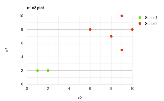
A scatter matrix, also known as a pair plot, is a powerful visualization tool in data analysis. It provides a grid of scatter plots that display relationships between pairs of variables in a dataset, helping engineers and data scientists to identify patterns, correlations, and potential outliers.

Read More: Scatter Plot Matrix

We calculate S_w  ( within the class scatter matrix ) and S_B ( between the class scatter matrix )  for the available data points.

S_W : To minimize variability within a class, inner class scatter.
S_B :  To increase between class variability, between class scatter.

scatter plot of the points

X1 = (y1, y2) ={ (2,2), (1,2), (1,2), (1,2), (2,2) } X2 = (y1,y2) ={ (9, 10), (6,8), (9,5), (8,7), (10,8) }

Within class scatter matrix:

[Tex]S_W = \sum_{i=1}^{c}S_i \\ S_i = \sum_{x\in D_i}^{c} (x-m_i)(x-m_i)^{T}[/Tex]

S_i is the class specific covariance matrix. m_i is the mean of individual class

Mean Calculation

We calculate the mean for each of the points present in the class. Here mean is the total sum of observations divided by the number of observations, we require this mean for calculating the covariance of the matrix.

[Tex]m_1 = [\frac{2+1+1+1+2}{5} , \frac{2+2+2+2+2}{5} ] \\  =  [1.4,2][/Tex]

[Tex]m_2 = [\frac{9+6+9+8+10}{5} , \frac{10+8+5+7+8}{5} ] \\  =  [8.4,7.6][/Tex]

Covariance matrix computation :
We subtract the mean value from each of the observation and then we calculate the average after performing the matrix multiplication with the transpose of the matrix.

Class specific covariance for the first class :

[Tex](X1-m_1) = \begin{bmatrix} 0.6 & -0.4 & -0.4 & -0.4 & 0.6\\ 0 & 0 & 0& 0& 0 \end{bmatrix}[/Tex]

[Tex]1) \begin{bmatrix} 0.6 \\ 0 \end{bmatrix} * \begin{bmatrix} 0.6 &0 \end{bmatrix} = \begin{bmatrix} 0.36 &0 \\ 0 &0 \end{bmatrix} \\\\ 2) \begin{bmatrix} -0.4 \\ 0 \end{bmatrix} * \begin{bmatrix} -0.4 &0 \end{bmatrix} = \begin{bmatrix} 0.16 &0 \\ 0 &0 \end{bmatrix} \\\\ 3) \begin{bmatrix} -0.4 \\ 0 \end{bmatrix} * \begin{bmatrix} -0.4 &0 \end{bmatrix} = \begin{bmatrix} 0.16 &0 \\ 0 &0 \end{bmatrix} \\\\ 4) \begin{bmatrix} -0.4 \\ 0 \end{bmatrix} * \begin{bmatrix} -0.4 &0 \end{bmatrix} = \begin{bmatrix} 0.16 &0 \\ 0 &0 \end{bmatrix} \\\\ 5) \begin{bmatrix} 0.6 \\ 0 \end{bmatrix} * \begin{bmatrix} 0.6 &0 \end{bmatrix} = \begin{bmatrix} 0.36 &0 \\ 0 &0 \end{bmatrix} \\\\[/Tex]

Averaging values from 1,2,3,4 and 5.
We calculate the sum of all the values for each element in the matrix for S1 and divide by the number of the observation which in the present computation is 5.

[Tex]matrix_{00} = \frac{ 0.36+0.16+0.16+0.16+0.36}{5}\\ =\frac{1.2}{5}\\ = 0.24\\\\ matrix_{01} = \frac{ 0+0+0+0+0}{5}\\ = 0\\\\ matrix_{10} = \frac{ 0+0+0+0+0}{5}\\ = 0\\\\ matrix_{11} = \frac{ 0+0+0+0+0}{5}\\ = 0\\\\[/Tex]

Therefore S₁ is :

[Tex]S_1 = \begin{bmatrix} 0.24 &0 \\ 0 &0 \end{bmatrix}[/Tex]

Class specific covariance for the second class :

[Tex](X2-m_2) = \begin{bmatrix} 0.6 & -2.4 & 0.6 & -0.4 & 1.6\\ 2.4 & 0.4 & -2.6& -0.6& 0.4 \end{bmatrix}[/Tex]

[Tex]1) \begin{bmatrix} 0.6 \\ 2.4 \end{bmatrix} * \begin{bmatrix} 0.6 &2.4 \end{bmatrix} = \begin{bmatrix} 0.36 &1.44 \\ 1.44 &05.76 \end{bmatrix} \\\\ 2) \begin{bmatrix} -2.4 \\ 0.4 \end{bmatrix} * \begin{bmatrix} -2.4 &0.4 \end{bmatrix} = \begin{bmatrix} 5.76 &-0.96 \\ -0.96 &0.16 \end{bmatrix} \\\\ 3) \begin{bmatrix} 0.6 \\ -2.6 \end{bmatrix} * \begin{bmatrix} 0.6 &-2.6 \end{bmatrix} = \begin{bmatrix} 0.36 &-1.56 \\ 1.56 &6.76 \end{bmatrix} \\\\ 4) \begin{bmatrix} -0.4 \\ -0.6 \end{bmatrix} * \begin{bmatrix} -0.4 &-0.6 \end{bmatrix} = \begin{bmatrix} 0.16 &0.24 \\ 0.24 &0.36 \end{bmatrix} \\\\ 5) \begin{bmatrix} 1.6 \\ 0.4 \end{bmatrix} * \begin{bmatrix} 1.6 &0.4 \end{bmatrix} = \begin{bmatrix} 2.56 &0.64 \\ 0.64 &0.16 \end{bmatrix} \\\\[/Tex]

Averaging values from 1,2,3,4 and 5
we calculate the sum of all the values for each element in the matrix for S2 and divide by the number of the observation which in the present computation is 5.

[Tex]matrix_{00} = \frac{ 0.36+5.76+0.36+0.16+2.56}{5}\\ =\frac{9.2}{5}\\ = 1.84\\\\ matrix_{01} = \frac{ 1.44-0.96-1.56+0.24+0.64}{5}\\ =\frac{-0.2}{5}\\ = -0.04\\\\ matrix_{10} = \frac{ 1.44-0.96-1.56+0.24+0.64}{5}\\ =\frac{-0.2}{5}\\ = -0.04\\\\ matrix_{11} = \frac{ 5.76+0.16+6.76+0.36+0.16}{5}\\ =\frac{13.2}{5}\\ = 2.64\\\\[/Tex]

Therefore S2 is :

[Tex]S_2 = \begin{bmatrix} 1.84 &-0.04 \\ -0.04 &2.64 \end{bmatrix}[/Tex]

Within class scatter matrix S_w :

S_W = S₁ + S₂

[Tex]S_W=  \begin{bmatrix} 0.24 &0 \\ 0 &0 \end{bmatrix} + \begin{bmatrix} 1.84 &-0.04 \\ -0.04 &2.64 \end{bmatrix} \\\\ =\begin{bmatrix} 2.08 &-0.04 \\ -0.04 &2.64 \end{bmatrix}[/Tex]

Between class scatter matrix S_B  :

[Tex]S_B = (m_1 – m_2) * (m_1 – m_2)^{T}\\\\ S_B = \begin{bmatrix} 7 & 5.6 \end{bmatrix} * \begin{bmatrix} 7 \\5.6 \end{bmatrix} \\\\ =\begin{bmatrix} 49 &37.2 \\ 37.2 &31.36 \end{bmatrix}[/Tex]

Total scatter matrix :

S_{T = SB + SW}

[Tex]S_w  =\begin{bmatrix} 49 &37.2 \\ 37.2 &31.36 \end{bmatrix} + \begin{bmatrix} 2.08 &-0.04 \\ -0.04 &2.64 \end{bmatrix} \\ =\begin{bmatrix} 51.08 & 37.16 \\ 37.16 &34 \end{bmatrix}[/Tex]

Therefore we have calculated between class scatter matrix and within class scatter matrix for the available data points.

We make use of these computations in feature extraction , where the main goal is to increase the distance between the class in the projection of points and decrease the distance between  the points within the class in the projection. Here we aim at generating data projection at the required dimension. 

Conclusion – Scatter Matrix

Scatter matrices are invaluable tools in engineering mathematics and data science, facilitating the exploration and analysis of complex datasets. They aid in identifying correlations, detecting outliers, and selecting features, ultimately enhancing the data modeling process.

Problem Solving on Scatter Matrix – FAQs

What is a scatter matrix used for?

A scatter matrix is used for visualizing pairwise relationships between multiple variables in a dataset, helping in identifying correlations, trends, and outliers.

How does a scatter matrix help in feature selection?

By showing correlations between variables, scatter matrices help in identifying redundant features, which can be removed to simplify models and improve performance.

Can scatter matrices detect non-linear relationships?

Yes, scatter matrices can reveal non-linear relationships between variables, aiding in the selection of appropriate machine learning models and feature transformations.

Why are scatter matrices useful in outlier detection?

They allow for the visual identification of outliers, which can then be addressed to improve the accuracy and robustness of predictive models.