Sequential data, often referred to as ordered data, consists of observations arranged in a specific order. This type of data is not necessarily time-based; it can represent sequences such as text, DNA strands, or user actions.

In this article, we are going to explore, sequential data analysis, it’s types and their implementations.

What is Sequential Data in Data Science?

Sequential data is a type of data where the order of observations matters. Each data point is part of a sequence, and the sequence’s integrity is crucial for analysis. Examples include sequences of words in a sentence, sequences of actions in a process, or sequences of genes in DNA.

Analyzing sequential data is vital for uncovering underlying patterns, dependencies, and structures in various fields. It helps in tasks such as natural language processing, bioinformatics, and user behavior analysis, enabling better predictions, classifications, and understanding of sequential patterns.

Types of Sequential Data

Sequential data comes in various forms, each with unique characteristics and applications. Here are three common types:

1. Time Series Data

Time series data consists of observations recorded at specific time intervals. This type of data is crucial for tracking changes over time and is widely used in fields such as finance, meteorology, and economics. Examples include stock prices, weather data, and sales figures.

2. Text Data

Text data represents sequences of words, characters, or tokens. It is fundamental to natural language processing (NLP) tasks such as text classification, sentiment analysis, and machine translation. Examples include sentences, paragraphs, and entire documents.

3. Genetic Data

Genetic data comprises sequences of nucleotides (DNA) or amino acids (proteins). It is essential for bioinformatics and genomic studies, enabling researchers to understand genetic variations, evolutionary relationships, and functions of genes and proteins. Examples include DNA sequences, RNA sequences, and protein sequences.

Sequential Data Analysis : Stock Market Dataset

Step 1: Import Libraries

Import necessary libraries for data handling, visualization, and time series analysis.

import pandas as pd
import matplotlib.pyplot as plt
import yfinance as yf
from statsmodels.tsa.seasonal import seasonal_decompose
from statsmodels.tsa.arima.model import ARIMA
from statsmodels.graphics.tsaplots import plot_acf, plot_pacf

Step 2: Load Data from Yahoo Finance

Download historical stock price data from Yahoo Finance. Replace ‘AAPL’ with the stock ticker of your choice.

# Load the dataset from Yahoo Finance
ticker = 'AAPL'
data = yf.download(ticker, start='2021-01-01', end='2024-07-01')

Output:

[*********************100%%**********************]  1 of 1 completed

Step 3: Select Relevant Column

Extract the ‘Close’ price column for analysis.

# Use the 'Close' column for analysis
df = data[['Close']]

Step 4: Plot the Time Series

Visualize the closing prices over time.

# Plot the time series
plt.figure(figsize=(10, 6))
plt.plot(df['Close'], label='Close Price')
plt.title(f'{ticker} Stock Price')
plt.xlabel('Date')
plt.ylabel('Close Price')
plt.legend()
plt.show()

Output:

Step 5: Decompose the Time Series

Decompose the time series into trend, seasonal, and residual components.

# Decompose the time series
decomposition = seasonal_decompose(df['Close'], model='additive', period=365)
fig = decomposition.plot()
fig.set_size_inches(10, 8)
plt.show()

Output:

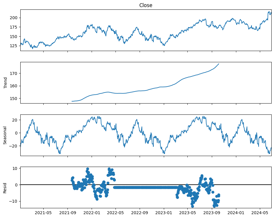Time series decomposed into trends, seasonal, and residual components

Step 6: Plot Autocorrelation and Partial Autocorrelation

Generate ACF and PACF plots to understand the correlation structure of the time series.

# Autocorrelation and Partial Autocorrelation Plots
plot_acf(df['Close'].dropna())
plt.show()

plot_pacf(df['Close'].dropna())
plt.show()

Output:

Autocorrelation Plot

Partial Autocorrelation Plot

Step 7: Fit an ARIMA Model

Define and fit an ARIMA model to the time series data.

# ARIMA Model
# Define the model
model = ARIMA(df['Close'].dropna(), order=(5, 1, 1))
# Fit the model
model_fit = model.fit()

# Summary of the model
print(model_fit.summary())

Output:

                               SARIMAX Results                                
==============================================================================
Dep. Variable:                  Close   No. Observations:                  877
Model:                 ARIMA(5, 1, 1)   Log Likelihood               -2108.273
Date:                Fri, 26 Jul 2024   AIC                           4230.545
Time:                        10:54:30   BIC                           4263.973
Sample:                             0   HQIC                          4243.331
                                - 877                                         
Covariance Type:                  opg                                         
==============================================================================
                 coef    std err          z      P>|z|      [0.025      0.975]
------------------------------------------------------------------------------
ar.L1          0.0082      5.467      0.002      0.999     -10.707      10.723
ar.L2         -0.0468      0.099     -0.473      0.637      -0.241       0.147
ar.L3         -0.0150      0.259     -0.058      0.954      -0.522       0.492
ar.L4          0.0068      0.084      0.081      0.935      -0.157       0.171
ar.L5         -0.0057      0.045     -0.126      0.899      -0.094       0.083
ma.L1          0.0091      5.466      0.002      0.999     -10.704      10.722
sigma2         7.2106      0.252     28.621      0.000       6.717       7.704
===================================================================================
Ljung-Box (L1) (Q):                   0.00   Jarque-Bera (JB):               173.60
Prob(Q):                              0.97   Prob(JB):                         0.00
Heteroskedasticity (H):               1.10   Skew:                             0.17
Prob(H) (two-sided):                  0.43   Kurtosis:                         5.15
===================================================================================

Step 8: Forecast Future Values

Use the fitted ARIMA model to forecast future values.

# Forecasting
# Forecast for the next 30 days
forecast_steps = 30
forecast = model_fit.forecast(steps=forecast_steps)

# Create a DataFrame for the forecast
forecast_dates = pd.date_range(start=df.index[-1], periods=forecast_steps + 1, freq='B')[1:]  # 'B' for business days



# Correcting the combination of forecast values and dates
forecast_combined = pd.DataFrame({
    'Date': forecast_dates,
    'Forecast': forecast
})

print(forecast_combined)

Output:

# Correcting the combination of forecast values and dates
forecast_combined = pd.DataFrame({
    'Date': forecast_dates,
    'Forecast': forecast
})

print(forecast_combined)

          Date    Forecast
877 2024-07-01  210.461277
878 2024-07-02  210.633059
879 2024-07-03  210.676056
880 2024-07-04  210.642225
881 2024-07-05  210.656179
882 2024-07-08  210.659306
883 2024-07-09  210.658497
884 2024-07-10  210.657659
885 2024-07-11  210.657931
886 2024-07-12  210.657926
887 2024-07-15  210.657903
888 2024-07-16  210.657897
889 2024-07-17  210.657905
890 2024-07-18  210.657904
891 2024-07-19  210.657904
892 2024-07-22  210.657904
893 2024-07-23  210.657904
894 2024-07-24  210.657904
895 2024-07-25  210.657904
896 2024-07-26  210.657904
897 2024-07-29  210.657904
898 2024-07-30  210.657904
899 2024-07-31  210.657904
900 2024-08-01  210.657904
901 2024-08-02  210.657904
902 2024-08-05  210.657904
903 2024-08-06  210.657904
904 2024-08-07  210.657904
905 2024-08-08  210.657904
906 2024-08-09  210.657904

Step 9: Plot the Forecast

Plot the forecasted values along with the original time series.

# Plot the forecast
plt.figure(figsize=(10, 6))
plt.plot(df['Close'], label='Historical')
plt.plot(forecast_combined['Date'], forecast_combined['Forecast'], label='Forecast', color='red')
plt.title(f'{ticker} Stock Price Forecast')
plt.xlabel('Date')
plt.ylabel('Close Price')
plt.legend()
plt.show()

Output:

AAPL Stock Price Forecast

Sequential Data Analysis using Sample Text

Step 1: Importing Necessary Libraries

This step involves importing the libraries required for text processing, sentiment analysis, and plotting.

import nltk
from nltk.tokenize import word_tokenize, sent_tokenize
from nltk.corpus import stopwords
from nltk.probability import FreqDist
from textblob import TextBlob
import matplotlib.pyplot as plt

Step 2: Downloading Necessary NLTK Data

Download the necessary datasets and models from NLTK to perform tokenization, stopwords removal, POS tagging, and named entity recognition.

nltk.download('punkt')
nltk.download('stopwords')
nltk.download('averaged_perceptron_tagger')
nltk.download('maxent_ne_chunker')
nltk.download('words')

Step 3: Sample Text

Define a sample text that will be used for all the analysis in this script.

text = """
Natural Language Processing (NLP) is a field of artificial intelligence 
that focuses on the interaction between computers and humans through 
natural language. The ultimate objective of NLP is to read, decipher, 
understand, and make sense of human languages in a valuable way. 
Most NLP techniques rely on machine learning to derive meaning from 
human languages.
"""

Step 4: Tokenization

Tokenize the sample text into words and sentences.

word_tokens = word_tokenize(text)
sentence_tokens = sent_tokenize(text)

Step 5: Remove Stopwords

Filter out common stopwords from the word tokens to focus on meaningful words.

stop_words = set(stopwords.words('english'))
filtered_words = [word for word in word_tokens if word.lower() not in stop_words and word.isalnum()]

Step 6: Word Frequency Distribution

Calculate and plot the frequency distribution of the filtered words

fdist = FreqDist(filtered_words)

plt.figure(figsize=(10, 5))
fdist.plot(30, cumulative=False)
plt.show()

Output:

Step 7: Sentiment Analysis

Perform sentiment analysis on the sample text using TextBlob to get the polarity and subjectivity.

blob = TextBlob(text)
sentiment = blob.sentiment

Step 8: Named Entity Recognition

Perform named entity recognition (NER) to identify entities like names, organizations, etc., in the text.

def named_entity_recognition(text):
    words = nltk.word_tokenize(text)
    tagged = nltk.pos_tag(words)
    entities = nltk.chunk.ne_chunk(tagged)
    return entities

entities = named_entity_recognition(text)

Step 9: Display Results

Print the results of the tokenization, filtered words, word frequency distribution, sentiment analysis, and named entities.

print("Word Tokens:", word_tokens)
print("Sentence Tokens:", sentence_tokens)
print("Filtered Words:", filtered_words)
print("Word Frequency Distribution:", fdist)
print("Sentiment Analysis:", sentiment)
print("Named Entities:")
entities.pprint()

Output:

Word Tokens: ['Natural', 'Language', 'Processing', '(', 'NLP', ')', 'is', 'a', 'field', 'of', 'artificial', 'intelligence', 'that', 'focuses', 'on', 'the', 'interaction', 'between', 'computers', 'and', 'humans', 'through', 'natural', 'language', '.', 'The', 'ultimate', 'objective', 'of', 'NLP', 'is', 'to', 'read', ',', 'decipher', ',', 'understand', ',', 'and', 'make', 'sense', 'of', 'human', 'languages', 'in', 'a', 'valuable', 'way', '.', 'Most', 'NLP', 'techniques', 'rely', 'on', 'machine', 'learning', 'to', 'derive', 'meaning', 'from', 'human', 'languages', '.']
Sentence Tokens: ['\nNatural Language Processing (NLP) is a field of artificial intelligence that focuses on the interaction between computers and humans through natural language.', 'The ultimate objective of NLP is to read, decipher, understand, and make sense of human languages in a valuable way.', 'Most NLP techniques rely on machine learning to derive meaning from human languages.']
Filtered Words: ['Natural', 'Language', 'Processing', 'NLP', 'field', 'artificial', 'intelligence', 'focuses', 'interaction', 'computers', 'humans', 'natural', 'language', 'ultimate', 'objective', 'NLP', 'read', 'decipher', 'understand', 'make', 'sense', 'human', 'languages', 'valuable', 'way', 'NLP', 'techniques', 'rely', 'machine', 'learning', 'derive', 'meaning', 'human', 'languages']
Word Frequency Distribution: <FreqDist with 30 samples and 34 outcomes>
Sentiment Analysis: Sentiment(polarity=0.012499999999999997, subjectivity=0.45)
Named Entities:
(S
  Natural/JJ
  Language/NNP
  Processing/NNP
  (/(
  (ORGANIZATION NLP/NNP)
  )/)
  is/VBZ
  a/DT
  field/NN
  of/IN
  artificial/JJ
  intelligence/NN
  that/WDT
  focuses/VBZ
  on/IN
  the/DT
  interaction/NN
  between/IN
  computers/NNS
  and/CC
  humans/NNS
  through/IN
  natural/JJ
  language/NN
  ./.
  The/DT
  ultimate/JJ
  objective/NN
  of/IN
  (ORGANIZATION NLP/NNP)
  is/VBZ
  to/TO
  read/VB
  ,/,
  decipher/RB
  ,/,
  understand/NN
  ,/,
  and/CC
  make/VB
  sense/NN
  of/IN
  human/JJ
  languages/NNS
  in/IN
  a/DT
  valuable/JJ
  way/NN
  ./.
  Most/JJS
  (ORGANIZATION NLP/NNP)
  techniques/NNS
  rely/VBP
  on/IN
  machine/NN
  learning/NN
  to/TO
  derive/VB
  meaning/NN
  from/IN
  human/JJ
  languages/NNS
  ./.)

Conclusion

In this article, we explored the concept of sequential data, which is crucial for various fields like natural language processing, bioinformatics, and user behavior analysis. We discussed different types of sequential data, including time series, text, and genetic data, highlighting their unique characteristics and applications. Additionally, we provided a practical example of sequential data analysis using a stock market dataset and textual data analysis.

Understanding and analyzing sequential data allows us to uncover patterns, dependencies, and structures that are essential for making informed decisions and predictions in various domains.