Principal coordinates analysis, or metric multidimensional scaling, is a statistical method employed to reconcile multivariate data to establish relationships based on similarities or dissimilarities. This kind of analysis aims to map the distance matrices of the original high-dimensional data space into a lower-dimensional data space where the distances between individual data points are preserved in a manner that maximizes. This method is more helpful when there are many and intricate relations between variables, like in ecological, genomic, and social scientific studies.

Introduction to Principal Coordinates Analysis

Principal Coordinates Analysis (PCoA) is a statistical method that converts data on distances between items into a map-based visualization of those items. Unlike Principal Component Analysis (PCA), which is based on Euclidean distances, PCoA can handle any distance or similarity measure, making it more flexible for various types of data.

• If we look at PCoA and PCA, we can notice that they both depend on the eigenvalue decomposition of matrices, but the eigenvalue analysis methods are different.
• PCoA gives primary importance to understanding the similarity among the objects; only then does it consider the similarity between the individual variables.

PCoA excels at analyzing data presented as dissimilarity matrices. These matrices capture the pairwise dissimilarities or distances between objects, making PCoA particularly valuable in fields like ecology, genetics, and social sciences where relationships are often expressed as distances rather than direct measurements.

The Mathematical Foundation: From Distances to Coordinates

At its core, PCoA aims to transform a dissimilarity matrix into a set of coordinates in a lower-dimensional space (typically 2D or 3D) while preserving the original distance relationships as faithfully as possible. This transformation is achieved through the following key steps:

1. Distance Matrix: First, calculate the distance between all pairs of districts. D of size ? × ? where Dij denote and stand for the separation of two points ? and j.

2. Double-Centering: To achieve this, add a weight matrix to the distance matrix such that the output will be a similarity matrix B using double-centering. This involves:

• Computing the centering matrix , where I is the identity matrix of the size of the matrix and 1 is a vector of ones.[Tex] J = I – \frac{1}{n} \mathbf{1} \mathbf{1}^T [/Tex]
• Applying J to therefore, the squared distance matrix [Tex] D^{(2)} = -\frac{1}{2} D^2 B = J D^{(2)} J [/Tex]

3. Eigen Decomposition: Perform an eigen decomposition of the similarity matrix B

[Tex] B = Q \Lambda Q^T [/Tex]

where Q is the eigenvector matrix and Λ is an identity matrix containing the eigenvalues on the diagonal.

4. Principal Coordinates: The principal coordinate values are derived by scaling the eigenvectors by the square root of the corresponding eigen values.

[Tex] X = Q \Lambda^{1/2} [/Tex]

Here, X is the matrix of coordinates of all the points in the new space, where the elements in the matrix are organised in rows.

5. Dimensionality Reduction: Usually, the selection of the top is performed in order to reduce the dimensionality that has been obtained. P Karl eigenvalues and eigenvectors that show most variability in data relative to lower dimensions.

How Does Principal Coordinates Analysis Work?

PCoA makes use of eigen analysis to find the main axes through a matrix. Then double centring is applied to the matrix (derived by eigenvalue decomposition). As a next step, it calculates a set of eigenvalues and eigenvectors, where each eigenvalue has an eigenvector.

The eigenvalues are ordered from the greatest to the least, and the first eigenvalue is considered the leading one. Using eigen vectors, one can explore or visualise the main axes through the initial distance matrix. Here, it doesn’t change the position of points related to each other but rather changes the coordinate system. The algorithm can be divided into following steps:

1. Transform the Distance Matrix: Computation of a distance matrix for the elements (eg: distance matrix).
2. Center the Matrix: Centering of the matrix.
3. Calculate Eigendecomposition: Eigen-decomposition of the centered distance matrix.
4. Project into Lower Dimensions: Scaling the eigenvectors.

Implementing Principal Coordinates Analysis Using skbio

In this section we make use of pcoa() method from scikit-bio for principal coordinate analysis.

Syntax:

skbio.stats.ordination.pcoa(distance_matrix, method='eigh',  number_of_dimensions=0, inplace=False)

Parameters:

• distance_matrix: A distance matrix
• method: The eigendecomposition method to perform PCoA. By default it uses SciPy’s eigh method
• number_of_dimensions: The dimension to reduce the distance matrix. By default it uses the number of dimensions of the distance matrix.
• inplace: If true, centers a distance matrix .

Returns: It returns an object that stores the PCoA results, including eigenvalues, the proportion explained by each of them, and transformed sample coordinates.

Example: We can create a dummy city distance dataset using pandas dataframe and let’s apply principal coordinate analysis to this dataset.

1. Importing Libraries:

import pandas as pd # for data manipulation from skbio.stats.ordination # perform PCoA import pcoaimport matplotlib.pyplot as plt # for plotting the result

2. Create a Dataset

data = [['Delhi', 0, 1000, 1700, 1500, 2500], ['Patna', 1000, 0, 1900, 1400, 2600], ['Goa', 1700, 1900, 0, 600, 750], ['Hyderabad', 1500, 1400, 600, 0, 1100], ['Kochi', 2500, 2600, 750, 1100, 0]] # Create the pandas DataFrame df = pd.DataFrame(data, columns=['Origin', 'Delhi', 'Patna', 'Goa','Hyderabad', 'Kochi'])

The above code creates a city distance dataset, which provides the distance between two cities in India.

3. Creating a Distance Matrix:

As a next step, we need to convert the pandas dataframe to distance matrix. Using to_numpy() method one can convert dataframe to matrix.

dmatrix = df.iloc[:,1:].to_numpy()

Here we remove the Origin column and the remaining columns are used for conversion.

4. Performing PCoA

pcoa_result = pcoa(dmatrix, number_of_dimensions=2)

The distance matrix calculated from the R and G channels is subjected to PCoA to achieve the dimensionality reduction while ensuring that the distances are preserved as much as possible.

5. Extracting Coordinates

coordinates = pcoa_result.samples

The coordinates from the Principal Coordinate Analysis are obtained as follows. These coordinates denote the points in the new lower-dimensional space as they are transformed.

6. Plotting the Results

df_pcoa = coordinates[['PC1', 'PC2']] df_pcoa['Origin'] = df['Origin'].to_numpy() df_pcoa = df_pcoa.set_index('Origin') print('\n\n', df_pcoa) fig, ax = plt.subplots() df_pcoa.plot('PC1', 'PC2', kind='scatter', ax=ax) plt.title('PCoA Plot') for k, v in df_pcoa.iterrows(): ax.annotate(k, v)

• The first two coordinates are then used to develop the scatter plot.
• The plot is termed PCoA Plot, and axis labels are represented by first and second principal coordinates.
• All points are labeled by their Origin name.

Now let’s implement the code and analyze the output. The code is as follows:

Output:

Dataframe Origin Delhi Patna Goa Hyderabad Kochi 0 Delhi 0 1000 1700 1500 2500 1 Patna 1000 0 1900 1400 2600 2 Goa 1700 1900 0 600 750 3 Hyderabad 1500 1400 600 0 1100 4 Kochi 2500 2600 750 1100 0 Distance Matrix [[ 0 1000 1700 1500 2500] [1000 0 1900 1400 2600] [1700 1900 0 600 750] [1500 1400 600 0 1100] [2500 2600 750 1100 0]] PCoA Result:: Ordination results: Method: Principal Coordinate Analysis (PCoA) Eigvals: 2 Proportion explained: 2 Features: N/A Samples: 5x2 Biplot Scores: N/A Sample constraints: N/A Feature IDs: N/A Sample IDs: '0', '1', '2', '3', '4'

Applying PCoA will create a set of new dimensions. Since we mentioned number of dimensions as 2, the code will create two new dimensions. The code to fetch the new coordinates as follows:

Output:

	PC1	PC2
0	-1056.345154	-536.888036
1	-1180.119143	455.976913
2	613.699911	-202.819152
3	237.635962	259.317403
4	1385.128424	24.412873

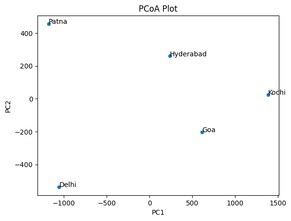
We can get the feature data from each coordinates. The code is as follows:

Python

print("First Principal Coordinates") print(coordinates['PC1'].values) print("\n Second Principal Coordinates") print(coordinates['PC2'].values)

Output:

First Principal Coordinates [-1056.34515353 -1180.11914341 613.69991135 237.63596197 1385.12842362] Second Principal Coordinates [-536.88803625 455.97691294 -202.81915198 259.3174025 24.41287279]

Visualization of PCoA Coordinates

Let’s plot both the coordinates along the x and y axis.

Python

df_pcoa = coordinates[['PC1', 'PC2']] df_pcoa['Origin'] = df['Origin'].to_numpy() df_pcoa = df_pcoa.set_index('Origin') fig, ax = plt.subplots() df_pcoa.plot('PC1', 'PC2', kind='scatter', ax=ax) plt.title('PCoA Plot') for k, v in df_pcoa.iterrows(): ax.annotate(k, v)

Output

PCoA plot

The result is a scatter plot in which five points are placed according to the values of the first two principal coordinates, which are determined during the PCoA. All the points on the plot are labeled based on the origin column and it has correct axis and title.

Explanation of the Plot:

• PCoA 1 and PCoA 2 Axes: These axes are the first two principal coordinates and they contain significant variance of the data set.
• Points and Labels: The points on the plot scale are the same number as the rows that are in the distance matrix above. The labels makes it easier to refer to specifically which point of view is being discussed.

Interpreting PCoA Plots: Untangling Complex Relationships

The resulting PCoA plot offers a visual representation of the original dissimilarity matrix. Here’s how to interpret it:

• Distance: The Euclidean distance between points in the PCoA plot approximates the original dissimilarity between the corresponding objects. Points that are close together are more similar, while points farther apart are more dissimilar.
• Dimensionality: The number of dimensions in the PCoA plot indicates the minimum number of dimensions needed to adequately represent the original dissimilarities. The first few dimensions usually capture the most significant variation in the data.
• Clusters: Groups or clusters of points in the PCoA plot can suggest the presence of distinct subgroups within the data.

Advantages and Limitations of PCoA

Advantages:

• Handles Dissimilarity Data: Uniquely suited for analyzing relationships expressed as distances, making it versatile for diverse data types.
• Dimensionality Reduction: Effectively summarizes complex relationships in a lower-dimensional space, aiding visualization and interpretation.
• Cluster Identification: Reveals potential groupings or subgroups within data based on similarity patterns.

Limitations:

• Non-Linear Relationships: May not accurately capture non-linear relationships between objects, as it assumes Euclidean distances.
• Sensitivity to Dissimilarity Measure: The choice of dissimilarity measure can significantly impact the results, so careful consideration is crucial.
• Interpretation: Requires domain knowledge to interpret the ecological or biological meaning of the axes in the PCoA plot.

Applications of Principal Coordinates Analysis

PCoA has a wide range of applications in various fields, including ecology, microbiology, and genomics. It is particularly useful for handling non-Euclidean distances, such as Bray–Curtis dissimilarity and unweighted UniFrac distance, which are commonly used in these fields to describe pairwise dissimilarity between samples. PCoA allows researchers to visualize variation across samples and potentially identify clusters by projecting the observations into a lower dimension. Few examples are given below:

• It helps to find a projection of the data that minimizes the differences between the distances in the original space and the distances in the lower-dimensional space.
• It facilitates visual inspection and exploration. The graphical representation of correlation provided by PCoA helps to explore their structure visually.
• PCoA helps to identify the dimensions that underlie the importance of similarity (or dissimilarity).
• It explains the dissimilarity based on the perceived difference between the two features.

Comparing PCoA with Other Multivariate Techniques: When to Use Which

Technique	Objective	Linearity	Data Type	Dimensionality Reduction	Interpretation
Principal Component Analysis (PCA)	Replace initial variables with orthogonal principal components	Linear	Continuous	Useful for dimensionality reduction	Aims to account for variances in the data
Principal Coordinates Analysis (PCoA)	Visualize pairwise distances between objects in a low-dimensional space	Non-linear	Continuous or metric	Useful for dimensionality reduction	Based on similarity-dissimilarity coefficients, aims to preserve original distances
Multidimensional Scaling (MDS)	Map objects to preserve dissimilarities in a low-dimensional space	Non-linear	Continuous or metric	Useful for dimensionality reduction	Based on similarity-dissimilarity coefficients, aims to preserve original distances
Cluster Analysis	Group similar data points into clusters	Non-linear	Depends on clustering algorithm	Useful for clustering and association analysis	Used for classification and segmentation, groups data into clusters
Correspondence Analysis (CA)	Examine co-occurrence frequencies of categories	Non-linear	Categorical	Useful for categorical data	Used to visualize relationships between categorical variables in low-dimensional space

Conclusion

Principal Coordinates Analysis (PCoA) is a versatile and powerful method for visualizing the similarities and dissimilarities among a set of objects. Its ability to handle various distance measures makes it suitable for a wide range of applications, from microbial ecology to marketing research. By understanding the mathematical foundations and practical implementation of PCoA, researchers can effectively use this technique to gain insights into their data.