Machine learning has revolutionized numerous industries, from healthcare to finance, by enabling the analysis of vast amounts of data and making predictions or decisions based on that data. However, this technology is not immune to the biases that exist in the data used to train it. These biases can lead to discriminatory outcomes, perpetuating existing social inequalities and causing harm to marginalized groups. It is crucial for developers, policymakers, and users to understand how bias creeps into machine learning systems and to implement strategies to mitigate and prevent it.

Understanding Bias in Machine Learning

Bias in machine learning occurs when the algorithms used to analyze data reflect and amplify the biases present in the data itself. This can happen at various stages of the machine learning process, including data collection, data preparation, model selection, and model deployment. Biased data can be the result of incomplete or unrepresentative datasets, biased assumptions in the algorithm development process, or the perpetuation of existing prejudices in the training data.

These biases can stem from various sources:

• Data Bias: This occurs when the training data reflects societal prejudices or historical imbalances. For instance, an algorithm trained on a dataset with a majority of male loan defaulters might be more likely to deny loans to future male applicants, even if their creditworthiness is similar to females.
• Algorithmic Bias: The choice of algorithm and its inherent assumptions can contribute to bias. For example, algorithms that rely on distance metrics might disadvantage groups geographically isolated from desired resources.
• Human Bias: The decisions made by humans throughout the ML pipeline, from data collection to feature engineering, can introduce bias. For instance, choosing features that perpetuate stereotypes can lead to discriminatory outcomes.

Identifying Bias in Machine Learning Models

Detecting bias in ML models requires a multi-pronged approach:

• Data Analysis: Analyzing the demographics of the training data can reveal imbalances. Statistical tests, like chi-square tests, can help identify statistically significant differences in how different groups are represented.
• Algorithmic Inspection: Understanding the model’s inner workings is crucial. Techniques like feature importance analysis can highlight features that disproportionately affect certain groups.
• Fairness Metrics: Metrics like fairness ratios and equality of opportunity scores can quantify bias by comparing model performance across different demographic groups.

Here’s an example of using fairness metrics:

Consider a loan approval model. We can calculate the True Positive Rate (TPR) – the proportion of truly creditworthy individuals approved for a loan – for different demographic groups. A significant disparity in TPR across groups would indicate potential bias.

To visualize a significant disparity in the True Positive Rate (TPR) across different demographic groups, we will highlight the differences in TPR and make it clear that disparities can indicate potential bias. For implementation. we will generate the dataset, calculate the TPR for each group, and visualize the results with a focus on indicating potential bias.

import pandas as pd
import numpy as np
import matplotlib.pyplot as plt
import seaborn as sns

# Generate a sample dataset
np.random.seed(42)
data_size = 1000

# Demographic groups and loan approval outcomes
age_group = np.random.choice(['Under 30', '30-50', 'Over 50'], size=data_size, p=[0.3, 0.5, 0.2])
income_level = np.random.choice(['Low', 'Medium', 'High'], size=data_size, p=[0.4, 0.4, 0.2])
creditworthy = np.random.choice([1, 0], size=data_size, p=[0.7, 0.3])  # 1: Creditworthy, 0: Not creditworthy
approved = np.random.choice([1, 0], size=data_size, p=[0.6, 0.4])  # 1: Approved, 0: Not approved

loan_df = pd.DataFrame({'AgeGroup': age_group, 'IncomeLevel': income_level, 'Creditworthy': creditworthy, 'Approved': approved})

# Function to calculate TPR
def calculate_tpr(df, group_col):
    tpr_data = []
    groups = df[group_col].unique()
    for group in groups:
        group_data = df[df[group_col] == group]
        tp = ((group_data['Creditworthy'] == 1) & (group_data['Approved'] == 1)).sum()
        fn = ((group_data['Creditworthy'] == 1) & (group_data['Approved'] == 0)).sum()
        tpr = tp / (tp + fn) if (tp + fn) > 0 else 0
        tpr_data.append({'Group': group, 'TPR': tpr})
    return pd.DataFrame(tpr_data)

# Calculate TPR for Age Groups
tpr_age = calculate_tpr(loan_df, 'AgeGroup')
# Calculate TPR for Income Levels
tpr_income = calculate_tpr(loan_df, 'IncomeLevel')

Plotting the TPR for different groups

# Plotting the TPR for different groups
plt.figure(figsize=(10,4))

plt.subplot(1, 2, 1)
sns.barplot(data=tpr_age, x='Group', y='TPR', palette='viridis')
plt.title('True Positive Rate by Age Group')
plt.ylabel('True Positive Rate')
plt.xlabel('Age Group')
for i, tpr in enumerate(tpr_age['TPR']):
    plt.text(i, tpr + 0.02, f'{tpr:.2f}', ha='center', va='bottom')

plt.subplot(1, 2, 2)
sns.barplot(data=tpr_income, x='Group', y='TPR', palette='viridis')
plt.title('True Positive Rate by Income Level')
plt.ylabel('True Positive Rate')
plt.xlabel('Income Level')
for i, tpr in enumerate(tpr_income['TPR']):
    plt.text(i, tpr + 0.02, f'{tpr:.2f}', ha='center', va='bottom')

plt.tight_layout()
plt.show()

# Highlighting potential bias
max_tpr_age = tpr_age['TPR'].max()
min_tpr_age = tpr_age['TPR'].min()
max_tpr_income = tpr_income['TPR'].max()
min_tpr_income = tpr_income['TPR'].min()

if max_tpr_age - min_tpr_age > 0.1:
    print(f"Potential bias detected in Age Group TPRs: Max TPR = {max_tpr_age:.2f}, Min TPR = {min_tpr_age:.2f}")

if max_tpr_income - min_tpr_income > 0.1:
    print(f"Potential bias detected in Income Level TPRs: Max TPR = {max_tpr_income:.2f}, Min TPR = {min_tpr_income:.2f}")

Output:

Fairness metrics

Mitigating Bias in Machine Learning Models

Once bias is identified, various techniques can be employed to mitigate its impact:

• Data Augmentation: This involves enriching the training data with synthetic examples or samples from underrepresented groups to improve representation. However, careful consideration is needed to avoid introducing artificial bias.
• Debiasing Techniques: These techniques aim to transform the data or model to reduce bias. For example, reweighting techniques can adjust the influence of individual data points to account for imbalances.
• Fairness-Aware Model Architectures: These models are specifically designed to promote fairness. For instance, adversarial training can involve creating an adversarial model that tries to identify and exploit the model’s biases, forcing the main model to learn fairer representations.

Let’s demonstrate how to apply reweighting to a dataset with imbalanced classes and visualize the impact of reweighting.

Imagine a dataset with a 90% majority class and a 10% minority class. Assigning a higher weight to minority class samples during training can encourage the model to focus on learning from the less frequent class and reduce bias against it.

We’ll create a synthetic dataset with an imbalanced class distribution, assign higher weights to the minority class, train a simple classifier, and visualize the impact of reweighting on class distribution in the model’s predictions.

Step 1: Train a model with imbalanced class distribution

import numpy as np
import matplotlib.pyplot as plt
from sklearn.datasets import make_classification
from sklearn.model_selection import train_test_split
from sklearn.linear_model import LogisticRegression
from sklearn.metrics import classification_report, ConfusionMatrixDisplay
import seaborn as sns

X, y = make_classification(n_samples=1000, n_features=8, n_informative=2, n_redundant=0,
                           n_clusters_per_class=1, weights=[0.9, 0.1], flip_y=0, random_state=42)
X_train, X_test, y_train, y_test = train_test_split(X, y, test_size=0.3, random_state=42)

# Calculate class weights
class_weights = {0: 1.0, 1: 9.0}  # Inverse of class frequencies

# Train a logistic regression model without class weights
model_no_weights = LogisticRegression()
model_no_weights.fit(X_train, y_train)
y_pred_no_weights = model_no_weights.predict(X_test)

# Train a logistic regression model with class weights
model_with_weights = LogisticRegression(class_weight=class_weights)
model_with_weights.fit(X_train, y_train)
y_pred_with_weights = model_with_weights.predict(X_test)

Step 2: Plotting the class distributions and reports

# Plot the class distribution in the predictions
plt.figure(figsize=(8, 4))

# Without reweighting
plt.subplot(1, 2, 1)
sns.countplot(x=y_pred_no_weights)
plt.title('Class Distribution without Reweighting')
plt.xlabel('Class')
plt.ylabel('Count')

# With reweighting
plt.subplot(1, 2, 2)
sns.countplot(x=y_pred_with_weights)
plt.title('Class Distribution with Reweighting')
plt.xlabel('Class')
plt.ylabel('Count')

plt.tight_layout()
plt.show()

# Print classification reports
print("Classification Report without Reweighting:")
print(classification_report(y_test, y_pred_no_weights))

print("Classification Report with Reweighting:")
print(classification_report(y_test, y_pred_with_weights))

Output:

Class distributions

Classification Report without Reweighting:
              precision    recall  f1-score   support

           0       0.98      0.99      0.99       273
           1       0.92      0.81      0.86        27

    accuracy                           0.98       300
   macro avg       0.95      0.90      0.92       300
weighted avg       0.98      0.98      0.98       300

Classification Report with Reweighting:
              precision    recall  f1-score   support

           0       0.99      0.96      0.97       273
           1       0.69      0.89      0.77        27

    accuracy                           0.95       300
   macro avg       0.84      0.92      0.87       300
weighted avg       0.96      0.95      0.96       300

Step 3: Confusion Matrix for Better Visualization

# Display confusion matrices for better visualization of model performance
fig, axes = plt.subplots(1, 2, figsize=(8, 4))

ConfusionMatrixDisplay.from_estimator(model_no_weights, X_test, y_test, ax=axes[0], cmap='Blues', values_format='d')
axes[0].set_title('Confusion Matrix without Reweighting')

ConfusionMatrixDisplay.from_estimator(model_with_weights, X_test, y_test, ax=axes[1], cmap='Blues', values_format='d')
axes[1].set_title('Confusion Matrix with Reweighting')

plt.tight_layout()
plt.show()

Output:

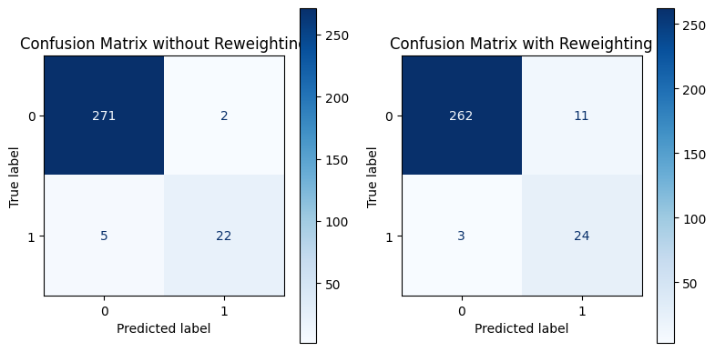Confusion Matrix

Preventing Bias in Machine Learning Pipelines

Proactive measures can be taken throughout the ML pipeline to prevent bias from creeping in:

• Diverse Teams: Building teams with diverse backgrounds and perspectives can help identify potential biases early on.
• Data Governance: Establishing procedures for data collection, cleaning, and labeling can minimize the introduction of human bias. Techniques like blind labeling, where the labeler is unaware of the data point’s origin, can be employed.
• Explainable AI (XAI): Developing models that are interpretable allows for a deeper understanding of how features and decisions contribute to the final outcome. This can help flag potential bias arising from the inner workings of the model.

Challenges and Considerations for Mitigating bias in ML

Mitigating bias in ML remains an ongoing challenge. Here are some key considerations:

• The No-Free-Lunch Theorem: There’s no single solution that works for all scenarios. The appropriate technique depends on the specific type of bias, data characteristics, and the desired fairness criteria.
• Data Privacy vs. Fairness: Techniques like data augmentation might raise concerns about data privacy. Balancing fairness with privacy is an important aspect of responsible AI development.
• Trade-offs Between Fairness and Performance: Sometimes, mitigating bias might lead to a slight decrease in model performance on the overall task. Determining the acceptable level of trade-off is crucial.

Case Studies and Examples

Case Study 1: Gender Bias in Recruitment

A recruitment algorithm was found to favor male candidates over female candidates due to biased training data. The company mitigated this bias by re-sampling the dataset to include more female candidates and using fairness metrics to evaluate the model.

Case Study 2: Gender Bias in Hiring Algorithms

A major tech company implemented an AI-powered hiring tool to screen job applicants. Over time, it was discovered that the algorithm was biased against female candidates, especially in technical roles. This bias originated from historical data that reflected a male-dominated industry and thus, the algorithm learned to favor male applicants.

Conclusion

Bias in machine learning is a critical issue that can lead to unfair and discriminatory outcomes. By understanding the types of bias, identifying their presence, and implementing strategies to mitigate and prevent them, we can develop fair and accurate ML models. Ensuring ethical considerations, forming diverse teams, and continuously monitoring models are essential steps in this process. By addressing bias, we can harness the full potential of machine learning while promoting fairness and equality.