No more manual copying and pasting data from one Google Sheet to another! Learn how to use the IMPORTRANGE function to effortlessly pull data from one sheet into another. In this article, you’ll discover how to use the IMPORTRANGE function step-by-step, making your data management smoother and more efficient.

Spreadsheet_url, range_string =IMPORTRANGE is the syntax for IMPORTRANGE.

IMPORT RANGE Function to Refer to Another Sheet

What is IMPORTRANGE and its formula?

Google Sheets is IMPORTRANGE, which is the best formula to use. It acts as a bridge, effortlessly transferring data from one spreadsheet (source) to another (destination); having any changes you make on the source sheet displayed promptly in the destination saves time and ensures that you are always working with the most recent data. Consider it a set-it-and-forget-it method for handling data in several spreadsheets!

The IMPORTRANGE syntax is:

=IMPORTRANGE(spreadsheet_url, range_string)

Here’s what those inputs refer to:

1. spreadsheet_url: The URL of the original spreadsheet with the data you want to bring into your new sheet
2. range_string: The area in the original spreadsheet containing the data you want to bring into your new sheet

How to use the IMPORTRANGE Function in Google Sheets

Step 1: Open the Browser

Open your preferred browser and go to “Google.”

Open the Browser

Step 2: Go to Google sheet

After clicking on Google, go to Google Workspace and scroll down to see “Google Sheets.”

Go to Google sheet

Step 3: Select the blank sheet

After clicking on Microsoft sheet, choose blank sheet and open it.

Select the blank sheet

Step 4: Click on the cell

Choose a cell where you want to apply this formula.

Click on the cell

Step 5: Copy the URL of sheet from which you need the data

Before putting Formulae, go on a spreadsheet whose data you want to copy, and copy the URL of that sheet.

Step 6: Back to a new sheet

After copying the URL from an old sheet, type Formulae in the new sheet you selected for this practice.

Step 7: Apply Formulae

Write the formula in a cell by typing =IMPORTARANGE and paste the URL you copied.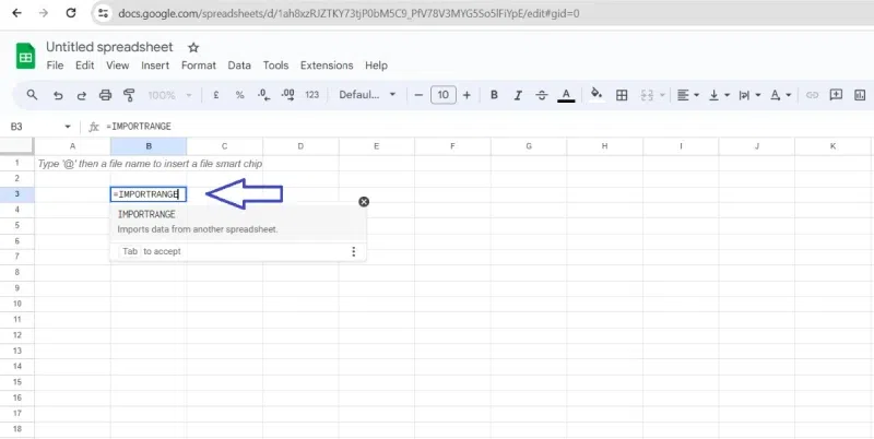

Apply Formulae

=IMPORTRANGE(“https://docs.google.com/spreadsheets/d/1LdPxJKzgw-cwnGcg2XYjdkbQtNN37oqrqDzoGw6E28k/edit#gid=1837330146”).

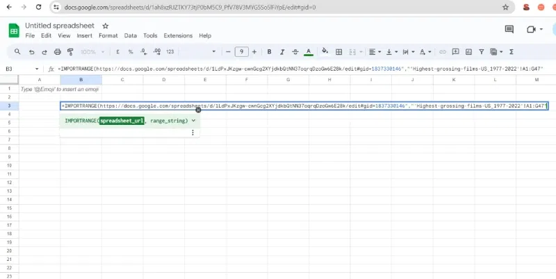Formula applied

Step 8: Build the range string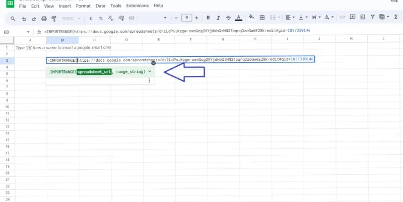

The range string uses this format: SheetName![top-left cell]:[bottom-right cell].

• SheetName: This is the name of the sheet containing your data. If it has spaces or numbers, enclose it in single quotes (‘).
• Top-left cell: This is the reference (e.g., A1) of the cell at the very beginning of the data area you want to copy.
• Bottom-right cell: This is the reference (e.g., G47) of the cell at the very end of the data area you wish to copy.

Example:

Imagine you want to import data from a “Sales Data” sheet in your original spreadsheet. The data starts in cell A1 and goes down to row 10, including columns A to C (so the bottom-right cell is C10).

Your range string for this example would be: ‘Sales Data’!A1:C10

Step 9: Using the Range String in Your Function

Using the Range String in Your Function

Once you have your range string, copy it and paste it into your function, surrounded by quotation marks (“). For instance, if you’re using the IMPORT RANGE function, it would look like this:

=IMPORTRANGE(“[Original Spreadsheet URL]”, “‘Sales Data’!A1:C10”)

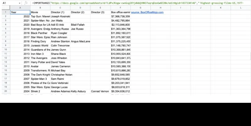Check your data

Note:

• Double-check your sheet names and cell references for accuracy.
• You can skip the single quotes if the sheet name is simple (without spaces or numbers).

Step 10: End your Command

If you close the bracket by putting parenthesis “)” and press enter, you will get a #REF error like the one below.

Step 11: Allow Access

Click “Allow access,” and your data will be imported. Your new spreadsheet will now display a duplicate of the data from your previous spreadsheet. However, the IMPORTRANGE function will still appear if you choose the cell where you wrote the function.

Benefits of IMPORTRANGE Formulae

• Conserve Time: Simplify the import of data from other spreadsheets.
• Simple Data Comparison: Compare data between sheets quickly and easily.
• Selective Data Import: Transfer particular rows from private files to safely shared documents.
• No Need for Extra Tools: Functions without third-party applications or browser plugins.
• Particular to Google Sheets: There needs to be a comparable feature in Excel.
• Quick Results: Receive real-time data updates.
• Minimize Errors: Steer clear of errors caused by manual copying and pasting.

Important Google Sheets functions to use with IMPORTRANGE

COUNTIF

COUNTIF will display the number of cells that satisfy the precise requirements you’re looking for inside a particular range. You can use this formula instead of scrolling through rows and rows of data to discover what you’re looking for.

How to use COUNTIF with IMPORTRANGE Function

Step 1: Type the formula

Start with =COUNTIF(.

Step 2: Choose your range

Inside the first parenthesis, specify the area you want to search. For example, A1:A50 would search cells A1 to A50.

Step 3: Set your criteria

Inside the second parenthesis, tell COUNTIF what to count.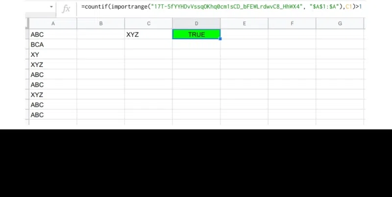

Countif with IMPORTRANG

Step 4: Press Enter

COUNTIF will show you how many cells match your criteria in that range.

How to Use VLOOKUP with Importrange

One of the best formulas for sorting through data is VLOOKUP. It may be used to locate relevant data, such as the pay of a specific employee or the quantity of sales a particular team produced in September. To put it briefly, data points can be easily compared.

=VLOOKUP(search_key, range, index, [is_sorted])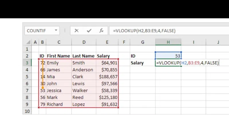

VLookup with Importange

How to use SPLIT with IMPORTRANGE

Step 1: Enter text

Enter the cell reference or text you want to split.

Step 2: Use “TEXTSPLIT” Formula

Use quotes around the character or string you want to use as the cutting tool (like “,” or a space).

Split with Importrange Function

Step 3: Optional extras

You can choose to split by each character (“,”) or only whole words (“) and even remove empty text after splitting.

Managing data imports from External files

IMPORTRANGE, among the best features in Google Sheets, can come to the rescue. IMPORTRANGE is much more happening than a digital copier. Rather than transferring data by hand, you link your spreadsheets together using a straightforward formula. Now, it’s as if whatever changes you make to the original data appear in the updated version. You can stop flipping between sheets and always have access to the most recent data.

IMPORT DATA (URL)

Enter the file’s URL (separated by quote marks) in those brackets to import data.

What distinguishes IMPORTRANGE from IMPORTDATA?

It allows you to import data between two Google Sheets and link them together. It is ideal if you frequently use data from another Google Sheet in your current one. It can import data from computer files such as HTML files (web pages), CSV files (popular for spreadsheets), and even XML files (a structured data format). It is helpful if your data still needs to be kept in a Google Sheet.

Conclusion

Using a straightforward formula, you can join spreadsheets without manually copying data between them. It gives you a superpower: your new spreadsheet will immediately reflect whatever modifications you make to the original data. There will be no more back-and-forth, and you’ll always have the most recent information available. These instructions will help you use IMPORTRANGE to keep your data structured across many Google Sheets and to optimize your workflow. You should also be aware of its restrictions.

FAQs on How to Use IMPORTRANGE in Google Sheets

Can I utilize spreadsheets other than Google Sheets using IMPORTRANGE?

I’m sorry, but IMPORTRANGE is limited to use with Google Sheets. The IMPORT DATA method should be used for data from external sources (such as CSV files).

Is there a maximum amount of data that I can import?

Although there’s no formal cap, massive datasets may impact performance. Consider utilizing different sheets if you are working with large amounts of data.