Clustering Distance Measures - Coding

Clustering is a fundamental concept in data analysis and machine learning, where the goal is to group similar data points into clusters based on their characteristics. One of the most critical aspects of clustering is the choice of distance measure, which determines how similar or dissimilar two data points are.

In this article, we will explore and delve into the world of clustering distance measures, exploring the different types, and their applications.

Table of Content

Why Distance Measures Matter?
Common Distance Measures
Choosing the Optimal Distance Metric for Clustering: Key Considerations
Choosing the Right Distance Measure

Why Distance Measures Matter?

Distance measures are the backbone of clustering algorithms. Distance measures are mathematical functions that determine how similar or different two data points are. The choice of distance measure can significantly impact the clustering results, as it influences the shape and structure of the clusters.

The choice of distance measure significantly impacts the quality of the clusters formed and the insights derived from them. A well-chosen distance measure can lead to meaningful clusters that reveal hidden patterns in the data, while a poorly chosen measure can result in clusters that are misleading or irrelevant.

Distance measurements specify how similarity between data points is assessed which makes them essential for grouping.
The performance of the clustering method, and its result can be strongly impacted by the distance measure selection.
It affects the formation of clusters and may have an impact on the validity and interpretability of the clusters.

Common Distance Measures

There are several types of distance measures, each with its strengths and weaknesses. Here are some of the most commonly used distance measures in clustering:

1. Euclidean Distance

The Euclidean distance is the most widely used distance measure in clustering. It calculates the straight-line distance between two points in n-dimensional space. The formula for Euclidean distance is:

[Tex]d(p,q)=\sqrt[]{\Sigma^{n}_{i=1}{(p_i-q_i)^2}}[/Tex]

where,

p and q are two data points
and n is the number of dimensions.

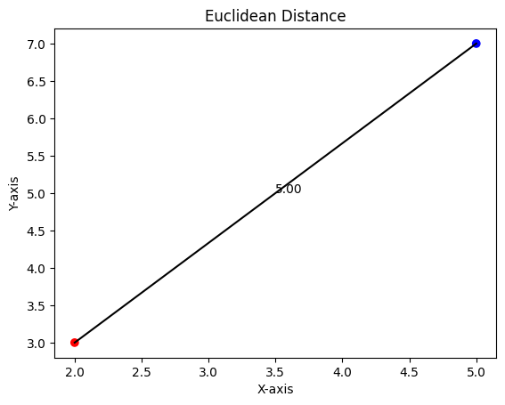
Utilizing Euclidean Distance

Python

import numpy as np
import matplotlib.pyplot as plt

# Calculate Euclidean distance
def euclidean_distance(point1, point2):
    return np.sqrt(np.sum((np.array(point1) - np.array(point2)) ** 2))

point1 = [2, 3]
point2 = [5, 7]
distance = euclidean_distance(point1, point2)
print(f"Euclidean Distance: {distance}")

# Plotting the points and the Euclidean distance
plt.figure()
plt.scatter(*zip(*[point1, point2]), color=['red', 'blue'])
plt.plot([point1[0], point2[0]], [point1[1], point2[1]], color='black')
plt.text((point1[0] + point2[0]) / 2, (point1[1] + point2[1]) / 2, f'{distance:.2f}', color='black')
plt.title('Euclidean Distance')
plt.xlabel('X-axis')
plt.ylabel('Y-axis')
plt.show()

Output:

Euclidean Distance: 5.0

Euclidean Distance

The two spots that we are computing the Euclidean distance between are represented by the red and blue dots in the figure. The Euclidean distance, represented by the black line that separates them is the distance measured in a straight line.

2. Manhattan Distance

The Manhattan distance, is the total of the absolute differences between their Cartesian coordinates, sometimes referred to as the L1 distance or city block distance. Envision maneuvering across a city grid in which your only directions are horizontal and vertical. The Manhattan distance, which computes the total distance traveled along each dimension to reach a different data point represents this movement. When it comes to categorical data this metric is more effective than Euclidean distance since it is less susceptible to outliers. The formula is:

[Tex]d(p,q)={\Sigma^{n}_{i=1}|p_i-q_i|}[/Tex]

Implementation in Python

Python

# Calculate Manhattan distance
def manhattan_distance(point1, point2):
    return np.sum(np.abs(np.array(point1) - np.array(point2)))

distance = manhattan_distance(point1, point2)
print(f"Manhattan Distance: {distance}")

# Plotting the points and the Manhattan distance
plt.figure()
plt.scatter(*zip(*[point1, point2]), color=['red', 'blue'])
plt.plot([point1[0], point1[0]], [point1[1], point2[1]], color='black', linestyle='--')
plt.plot([point1[0], point2[0]], [point2[1], point2[1]], color='black', linestyle='--')
plt.text((point1[0] + point2[0]) / 2, (point1[1] + point2[1]) / 2, f'{distance:.2f}', color='black')
plt.title('Manhattan Distance')
plt.xlabel('X-axis')
plt.ylabel('Y-axis')
plt.show()

Output:

Manhattan Distance: 7

Manhattan Distance

The two points are represented by the red and blue points in the plot. The grid-line-based method used to determine the Manhattan distance is depicted by the dashed black lines.

3. Cosine Similarity

Instead than concentrating on the exact distance between data points , cosine similarity measure looks at their orientation. It calculates the cosine of the angle between two data points, with a higher cosine value indicating greater similarity. This measure is often used for text data analysis, where the order of features (words in a sentence) might not be as crucial as their presence. It is used to determine how similar the vectors are, irrespective of their magnitude.

[Tex]{similarity(A,B)}=\frac{A.B}{\|A\|\|B\|}[/Tex]

Example in Python

Python

# Calculate Cosine Similarity
def cosine_similarity(point1, point2):
    dot_product = np.dot(point1, point2)
    norm1 = np.linalg.norm(point1)
    norm2 = np.linalg.norm(point2)
    return dot_product / (norm1 * norm2)

distance = cosine_similarity(point1, point2)
print(f"Cosine Similarity: {distance}")

# Plotting the points and the Cosine similarity
# For Cosine Similarity, we will plot the vectors originating from the origin
origin = [0, 0]
plt.figure()
plt.quiver(*origin, *point1, angles='xy', scale_units='xy', scale=1, color='red')
plt.quiver(*origin, *point2, angles='xy', scale_units='xy', scale=1, color='blue')
plt.xlim(0, max(point1[0], point2[0]) + 1)
plt.ylim(0, max(point1[1], point2[1]) + 1)
plt.title('Cosine Similarity')
plt.xlabel('X-axis')
plt.ylabel('Y-axis')
plt.show()

Output:

Cosine Similarity: 0.9994801143396996

download-(2)

In the plot, the red and blue arrows represent the vectors of the two points from the origin. The cosine similarity is related to the angle between these vectors.

4. Minkowski Distance

Minkowski distance is a generalized form of both Euclidean and Manhattan distances, controlled by a parameter p. The Minkowski distance allows adjusting the power parameter (p). When p=1, it’s equivalent to Manhattan distance; when p=2, it’s Euclidean distance.

[Tex]d(x,y)=(\Sigma{^{n}_{i=1}}|x_i-y_i|^p)^\frac{1}{p}[/Tex]

Utilizing Minkowski Distance

Python

# Calculate Minkowski distance
def minkowski_distance(point1, point2, p):
    return np.power(np.sum(np.abs(np.array(point1) - np.array(point2)) ** p), 1/p)

p = 3
distance = minkowski_distance(point1, point2, p)
print(f"Minkowski Distance (p={p}): {distance}")

# Plotting the points and the Minkowski distance
plt.figure()
plt.scatter(*zip(*[point1, point2]), color=['red', 'blue'])
# For Minkowski with p=3, the visualization isn't straightforward like Euclidean or Manhattan
# We will plot the same line for illustration purposes
plt.plot([point1[0], point2[0]], [point1[1], point2[1]], color='black')
plt.text((point1[0] + point2[0]) / 2, (point1[1] + point2[1]) / 2, f'{distance:.2f}', color='black')
plt.title('Minkowski Distance')
plt.xlabel('X-axis')
plt.ylabel('Y-axis')
plt.show()

Output:

Minkowski Distance (p=3): 4.497941445275415

Minkowski Distance

In the plot, the visualization is similar to Euclidean distance when p=3, but the distance calculation formula changes.

5. Jaccard Index

This measure is ideal for binary data, where features can only take values of 0 or 1. It calculates the ratio of the number of features shared by two data points to the total number of features. Jaccard Index measures the similarity between two sets by comparing the size of their intersection and union.

[Tex]J(A,B)=\frac{|A\cap B|}{|A\cup B|}[/Tex]

Jaccard Index Example in Python

Python

from sklearn.metrics import jaccard_score

# Define two binary vectors
vector1 = np.array([1, 1, 0, 0])
vector2 = np.array([1, 1, 1, 0])

# Calculate Jaccard index
jaccard_index = jaccard_score(vector1, vector2)
print("Jaccard Index:", jaccard_index)

Output:

Jaccard Index: 0.6666666666666666

Choosing the Optimal Distance Metric for Clustering: Key Considerations

The type of data and the particulars of the clustering operation will determine which distance metric is best. Here are some things to think about:

Data Type: Different distance metrics may be needed for binary, categorical , or numerical data.
Scale Sensitivity: The scale of the data affects the measurement of some distances such as Euclidean distance. Data standardization can aid in resolving this problem.
Interpretability: For the specified application the selected measure should yield findings , that are both meaningful and comprehensible.
Computational Efficiency: Take into account the complexity of computing particularly when working with big datasets.
Existence of Outliers: Outliers have a big impact on metrics based on distance. If outliers are an issue use metrics that are less susceptible to them.
Clustering Algorithm: Various clustering methods may need a certain distance metric.

Choosing the Right Distance Measure

The choice of distance measure depends on the nature of the data and the clustering algorithm being used. Here are some general guidelines:

Euclidean distance is suitable for continuous data with a Gaussian distribution.
Manhattan distance is suitable for data with a uniform distribution or when the dimensions are not equally important.
Minkowski distance is suitable when you want to generalize the Euclidean and Manhattan distances.
Cosine similarity is suitable for text data or when the angle between vectors is more important than the magnitude.
Jaccard similarity is suitable for categorical data or when the intersection and union of sets are more important than the individual elements.

Conclusion

Distance measures are the backbone of clustering algorithms. It is essential to comprehend clustering distance measurements in order to analyze data effectively. You can improve your clustering algorithms accuracy and insights by using the right distance measure. Understanding how to quantify similarity will have a big influence on your outcomes whether you’re working with text, photos , or quantitative data. Remember these ideas and methods as you investigate clustering further to help you make wise choices and get better results for your data science endeavors.

Reffered: https://www.geeksforgeeks.org

AI ML DS

Related
Jobs related to R Programming
MultiLabel Classification using CatBoost
Sys.sleep() Function in R : Timed Execution Pauses
Accelerating LightGBM: Harnessing Parallel and GPU Training
NLP Full Form

Type:	Geek
Category:	Coding
Sub Category:	Tutorial
Uploaded by:	Admin
Views:	15