In this article, we are going to learn about the topic of principal component analysis for dimension reduction using R Programming Language. In this article, we also learn the step-by-step implementation of the principal component analysis using R programming language, applications of the principal component analysis in different fields, and its advantages and disadvantages. Before discussing the principal component analysis, we discuss a few pre-requisite topics related to the principal component analysis.

What is Dimensionality Reduction ?

Dimension reduction is the process of reducing the number of dimensions and reducing the variable available by considering a few essential features. It can also defined as the technique that converts the large-dimension dataset to the small-dimension data set by considering the essential features. The dimensions reduction technique is mainly used when we are dealing with a large amount of data set. The few methods in dimension reduction are principal component analysis, wavelet transforms, singular value decomposition, linear discriminant analysis, generalized discriminant analysis, and many more.

What is Principal Component Analysis ?

Principal component analysis is a useful and an important method for the dimensionality reduction in the data pre processing . Principal Component analysis is served as a unsupervised dimensionality reduction technique . In the principal component analysis we almost consider the variance of the data points , without considering the other class labels . We reduce the data based on the variance of the data points without considering the other class labels or dependent variable in the provided information .

Steps in Principal Component Analysis

These are the few steps in principal component analysis

1. Standardization of the data of the given input data.
2. Calculation of the covariance matrix for the standardized data.
3. Calculating the eigen values and eigen vectors for the covariance matrix.
4. Sorting the eigen values and eigen vectors .
5. Identify the principal components and create a feature for the data.
6. Project the data on to the principal component axes.

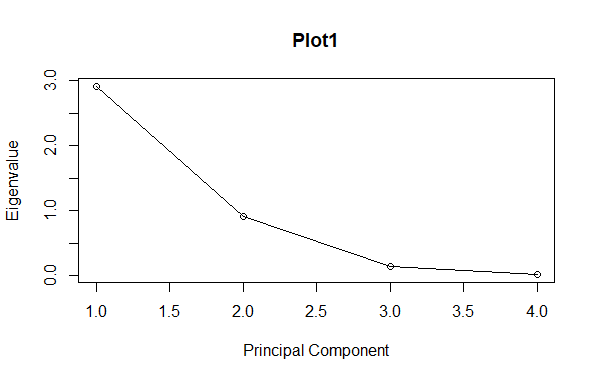
Example of Principal Component Analysis

In this section , we discuss an example how to solve the principal component analysis mathematically.

Let us take the data matrix as [Tex]a = \left[\begin{array}{cc} 1 & 4\\ 2 & 5 \\ 3 & 6 \\ \end{array}\right][/Tex]

Now let us standardize the matrix by claculating the mean for the each column and subtracting the each data point from the mean of the each column.

Now , [Tex]mean\;column1=(1+2+3)/3[/Tex] = 2

[Tex]mean\;column2=(4+5+6)/3[/Tex] = 5

Now the matrix a becomes like this [Tex]a_{standrard} = \left[\begin{array}{cc} 1 – 2 & 4-5\\ 2 – 2 & 5-5 \\ 3 – 2 & 6-5 \\ \end{array}\right][/Tex]

[Tex]a_{standrard} = \left[\begin{array}{cc} -1 & -1 \\ 0 & 0 \\ 1 & 1 \\ \end{array}\right][/Tex]

Now the covariance matrix for the matrix a will be [Tex]a_{cov}= \left[\begin{array}{cc} 1 & 1 \\ 1 & 1 \\ \end{array}\right][/Tex]

Now let us calculate the eigen values and eigen vectors for the above covariance matrix :

For eigen values

[Tex]| {a_{cov} – \lambda I }|= 0[/Tex] i.e., det([Tex]a-\lambda I[/Tex])=0

[Tex]\left|\begin{array}{cc} 1 – \lambda & 1 \\ 1 & 1 – \lambda \\ \end{array}\right|=0[/Tex]

[Tex](1 – \lambda )^2 – 1 = 0[/Tex]

[Tex]1 + \lambda^2 – 2\lambda – 1 = 0[/Tex]

[Tex] \lambda^2 – 2\lambda = 0[/Tex]

[Tex]\lambda (\lambda – 2) = 0[/Tex]

\lambda = 0,\lambda = 2 are the eigen values for the matrix .

[Tex]eigen\_values = \left[\begin{array}{cc} 0 \\ 2 \\ \end{array}\right][/Tex]

For eigen vectors

From eigen value 0

[Tex]\left[\begin{array}{cc} 1 – 0 & 1 \\ 1 & 1 – 0 \\ \end{array}\right]\left[\begin{array}{cc} x_1 \\ x_2 \\ \end{array}\right] = 0[/Tex]

[Tex]eigen\_vector = \left[\begin{array}{cc} – 1 \\ 1 \\ \end{array}\right][/Tex]

From eigen value 2

[Tex]\left[\begin{array}{cc} 1 – 2 & 1 \\ 1 & 1 – 2 \\ \end{array}\right]\left[\begin{array}{cc} x_1 \\ x_2 \\ \end{array}\right] = 0[/Tex]

[Tex]eigen\_vector = \left[\begin{array}{cc} 1 \\ 1 \\ \end{array}\right][/Tex]

Let us now sort the eigen values in the decreasing order

[Tex]eigen\_values = \left[\begin{array}{cc} 2 \\ 0 \\ \end{array}\right][/Tex]

Choose eigen vector values for the top k eigen values .In this case we are selecting the value for the K is 2 . K is also called as the principal components . Hence the final matrix becomes the [Tex]resultant\_matrix = \left[\begin{array}{cc} 1 & – 1 \\ 1 & 1 \\ \end{array}\right][/Tex] .

The above resultant matrix is the dimensions reduced data for the given data . In this way we can use the steps of the principal component analysis for dimensionality reduction.

Implementation of the principle component analysis using R

Step-1 : Loading the input data

In order to implement the principle component analysis for dimension reduction using R , firstly we need the input data . In this example we are going to use the iris data set which have the 150 rows and 5 columns. In iris data set the last column has the class label shows the type of species.

Output:

Sepal.Length Sepal.Width Petal.Length Petal.Width Species
Min. :4.300 Min. :2.000 Min. :1.000 Min. :0.100 setosa :50
1st Qu.:5.100 1st Qu.:2.800 1st Qu.:1.600 1st Qu.:0.300 versicolor:50
Median :5.800 Median :3.000 Median :4.350 Median :1.300 virginica :50
Mean :5.843 Mean :3.057 Mean :3.758 Mean :1.199
3rd Qu.:6.400 3rd Qu.:3.300 3rd Qu.:5.100 3rd Qu.:1.800
Max. :7.900 Max. :4.400 Max. :6.900 Max. :2.500

In the above code we just loaded the input data by using the function read.csv() and stored in the variable mydata, in the second line we just printed the stored data and finally we used a summary() function to print the summary of the data.To know more about the summary and read.csv() we can refer to the link provided summary() and read.csv() .

Step – 2 : Standardization of the data of the given input data

Standardization of data is the process of converting the data point to common format , which makes the data analyzing process easy. In this standardization process we used the process scaling to reduce the last column of the mydata . Let us now look at the code in r programming to remove the last row of the iris data which is class label which determines the type of species .

Output:

Sepal.Length Sepal.Width Petal.Length Petal.Width
[1,] -0.8976739 1.01560199 -1.335752 -1.311052
[2,] -1.1392005 -0.13153881 -1.335752 -1.311052
[3,] -1.3807271 0.32731751 -1.392399 -1.311052
[4,] -1.5014904 0.09788935 -1.279104 -1.311052
[5,] -1.0184372 1.24503015 -1.335752 -1.311052
[6,] -0.5353840 1.93331463 -1.165809 -1.048667

In the above code we just made the data set standardized . We have removed last row of the mydata as we are the working with unsupervised principal component analysis , as the usupervised techniques does not require the class labels.In the above we just used the scale() function . Sacle() is a function which is a built in R function which is used for the scaling and centering the values of a matrix.To know more about the scale() function we can refer to the link provided scale() function .

Step – 3 : Covariance matrix calculation

Covariance matrix is a matrix of values of covariance between pair of elements of a random sample . Covariance matrix is a square matrix . We know that the principal component analysis uses the variance as a main consideration , we are calculating the covariance matrix . Let us look at the R programming code for the calculation of the covariance matrix.

Output:

Sepal.Length Sepal.Width Petal.Length Petal.Width
Sepal.Length 1.0000000 -0.1175698 0.8717538 0.8179411
Sepal.Width -0.1175698 1.0000000 -0.4284401 -0.3661259
Petal.Length 0.8717538 -0.4284401 1.0000000 0.9628654
Petal.Width 0.8179411 -0.3661259 0.9628654 1.0000000

In the above code we just created the covariance matrix and stored in the variable covarincematrix and in the next line of the code we just printed the covarince matrix.In the code we have used the function cov() for the calculation of the covariance matrix . cov() function is a built in R programming function for the calculation of the covariance matrix. To know ore about the cov() function we can refer to the link provided cov() .

Step – 4 : Calculating the eigen values and eigen vectors

Eigen values are the scalar values which are associated with the set of linear equations in linear transformation. Eigen vector is a vector of scalar values which are also called as characteristic values . Let us now look at the code for the calculation of eigen values and eigen vectors .

Output:

eigen() decomposition
$values
[1] 2.91849782 0.91403047 0.14675688 0.02071484

$vectors
[,1] [,2] [,3] [,4]
[1,] 0.5210659 -0.37741762 0.7195664 0.2612863
[2,] -0.2693474 -0.92329566 -0.2443818 -0.1235096
[3,] 0.5804131 -0.02449161 -0.1421264 -0.8014492
[4,] 0.5648565 -0.06694199 -0.6342727 0.5235971

In the above code we have used the eigen() function to calculate the eigen values and eigen vectors . Eigen() is a built in function in R programming to calculate the eigen values and eigen vectors of the given matrix.

Step – 5 : Sorting the eigen values and eigen vectors

In the below code we are just sorting the eigen values and eigen vectors by using the function order . Order() is also a built in function that arranges the provided data in the form of ascending or descending order .

Output:

[1] 2.91849782 0.91403047 0.14675688 0.02071484


[,1] [,2] [,3] [,4]
[1,] 0.5210659 -0.37741762 0.7195664 0.2612863
[2,] -0.2693474 -0.92329566 -0.2443818 -0.1235096
[3,] 0.5804131 -0.02449161 -0.1421264 -0.8014492
[4,] 0.5648565 -0.06694199 -0.6342727 0.5235971

Step – 6 : Select principal components and project on to the data

In this step we are going to select the principal components and reducing the data as per the selected principal components. Let us look at the code for it .

Output:

[,1] [,2]
[1,] 0.5210659 -0.37741762
[2,] -0.2693474 -0.92329566
[3,] 0.5804131 -0.02449161
[4,] 0.5648565 -0.06694199

[,1] [,2]
[1,] -2.25714118 -0.478423832
[2,] -2.07401302 0.671882687
[3,] -2.35633511 0.340766425
[4,] -2.29170679 0.595399863
[5,] -2.38186270 -0.644675659

Step – 7 : Interpreting the results

In this step we are going to plot the principal component analysis graphs using the plot function.

Output:

[1] 0.729624454 0.228507618 0.036689219 0.005178709

Principal Component Analysis for dimension reduction using R

Visualization of reduced dimensional data

Output:

Principal Component Analysis for dimension reduction using R

Applications of Principal Component Analysis

Principal Component Analysis is not only used in data preprocessing , it has many applications over many fields like data science , machine learning , data mining , economics , finance and many more .

1. Principal Component Analysis techniques is used for the dimensionality reduction by using the component variability .
2. Principal Component Analysis makes the data visualization more simple by reducing the higher dimensions to lower dimensions which reveals the data patterns ,trends and clusters.
3. In machine learning and predictive modelling principal component analysis is used for the feature engineering , which is feature extraction and feature selection.
4. Principal component analysis reduces the noise , as it calculates the siginificant value of the variance of data points.
5. Principal component analysis can be used in the image processing for the compression of images . In this process the image is represnted in the form of principal components.
6. It can be used in the economica and finance for the analyszing the reasons for the prices changes .
7. In speech recognization , principal component analysis is used for the pattern recognition and efficient processing of the data or signal.
8. Principal component analysis can be used in quality control , remote sensing , medical imaging and computer vision for the reduction of data and analyze the different data.

Advantages of principal component analysis

1. Principal component analysis is more efficient for computations.
2. It can be useful for the dimensionality reducton by considering important variables.
3. It is helpful for the noise reduction and feature extraction.
4. It can also has the advantage of feature selection and data visualization by reducing the dimensions of the data.
5. Principal component analysis can be used for the conversion of original variables to the uncorelated variables .
6. It improves the model performance by reducing the causes of the overfitting .
7. It helps in preprocessing the data in machine learning , data mining and data science algorithms .
8. Principal component analysis has the capability to find the important variables.

Disadvantages of principal component analysis

1. Principal component analysis sometimes not suitable for the categorical or qualitative data.
2. Principal component analysis is not robust to non normal data .
3. Principal component analysis will not consider the small value of variance.
4. It has a difficulty in determining the number of components to consider for the reduction.
5. This technique is sensitive to outliers and depend on the property of scaling .
6. As it does not consider the lower variance values , in such cases most important information may lost.

Conclusion

In conclusion , principal component analysis plays a major role in the dimensionality reduction . In this article we have learned the basic concepts of the principal component analysis , its implementation in r programming , its applications in different fields , advantages and disadvantages.