Excel provides powerful functions to find the top or bottom N values in a dataset, making data analysis much easier. The functions used to find the Nth largest and Nth smallest numbers are =LARGE(array, k) and =SMALL(array, k), respectively. In this article, we will explore how to use these functions effectively, along with a deeper understanding of cell references.

How to find Top or Bottom N values in Excel?

Understanding Cell Reference 

Before understanding the LARGE and SMALL functions. We first need to have a fine knowledge of cell references. A cell reference is of two types: 

1. Relative Reference 

Relative reference is the reference that changes with cells.

1. If we try dragging the same formula down across a column then numbers will increase.
2. If we try dragging the same formula side across a row, then the alphabets will increase. 

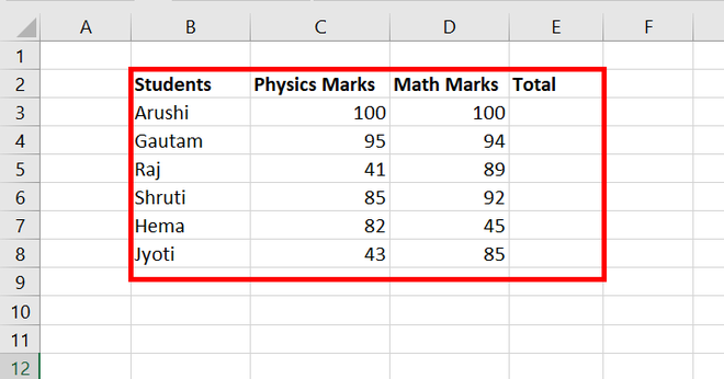
Example: Calculating Total Marks:

Consider a data set of Students with their Physics and Math marks. Calculate the total marks. 

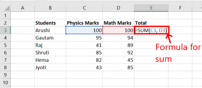
Steps for finding the total with Relative Reference

Step 1: Write a formula for sum i.e. “= SUM(value1, value2)” and press Enter. 

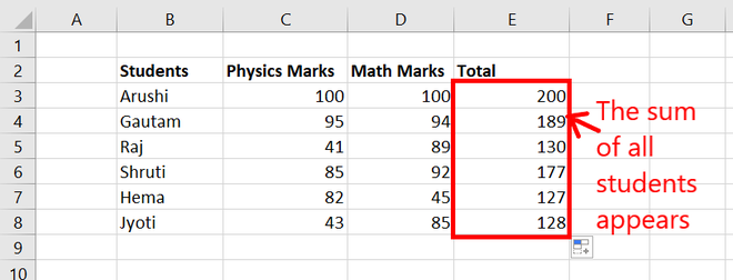
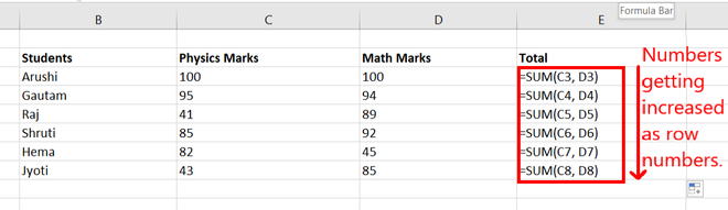
Step 2: Try dragging the same formula downward and hence we get the sum of all students. 

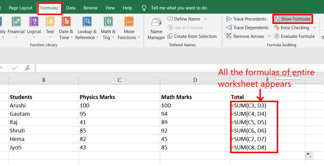
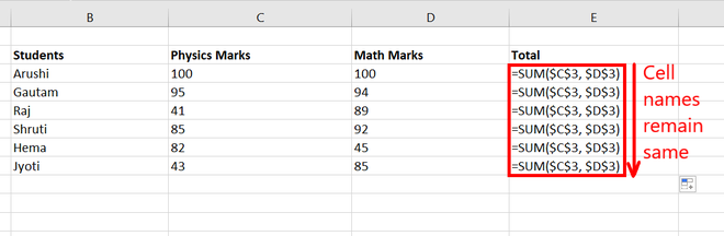
Step 3: Go to Formula Tab and click on Show Formulas. Now, all the formulas of the given worksheet will appear. 

Step 4: We find in range E3:E9 that the values inside the functions are increasing as we go downward in a row. For Example: in cell E3, the formula is =SUM(C3, D3) and in cell E4, the formula is =SUM(C4, D4). 

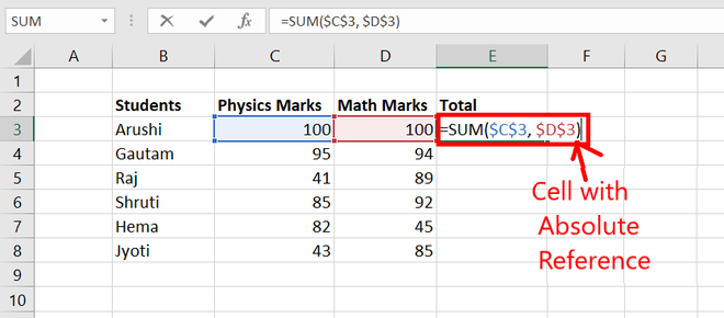
2. Absolute Reference 

The absolute reference remains static even if the rows or columns are changing. There can be two ways to make a selected cell with absolute reference:

1. Use $ symbol: Write $ after each and every character of the selected cells.
2. Use F4: Press Fn + F4 on your keyboard to make absolute reference to a selected cell.

Consider the same data set as above. Try using the same formula for total but with absolute reference. 

Steps of finding total with absolute reference

Step 1: Considering the same data set and write the function with absolute reference. 

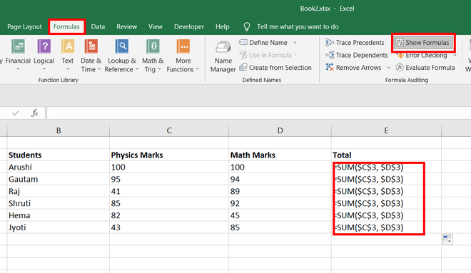
Step 2: Now, go to Formulas Tab and click on Show Formulas. All formulas of the given worksheet appear. 

Step 3: We observe that while going downward in a row the selected cells remain the same. 

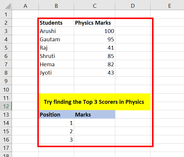
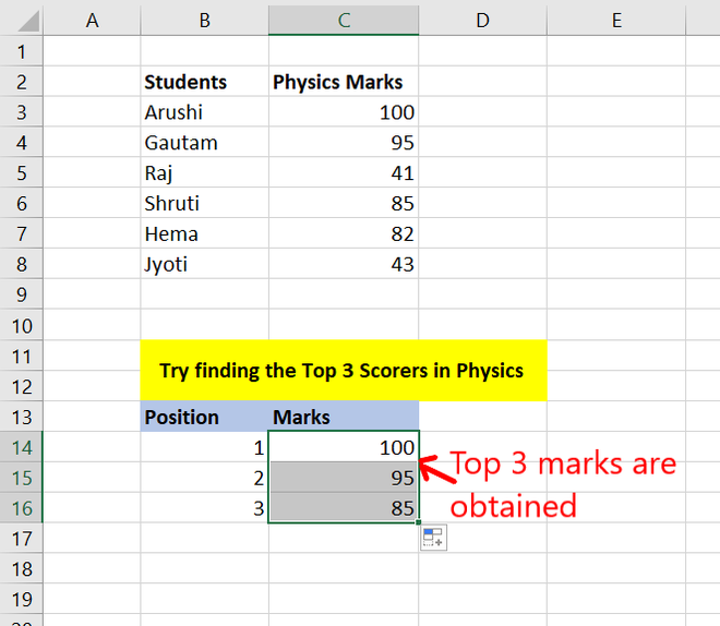
How to Find Top N values in Excel

Given a data set of Students and their Marks. Try finding the highest 3 marks scored by students. 

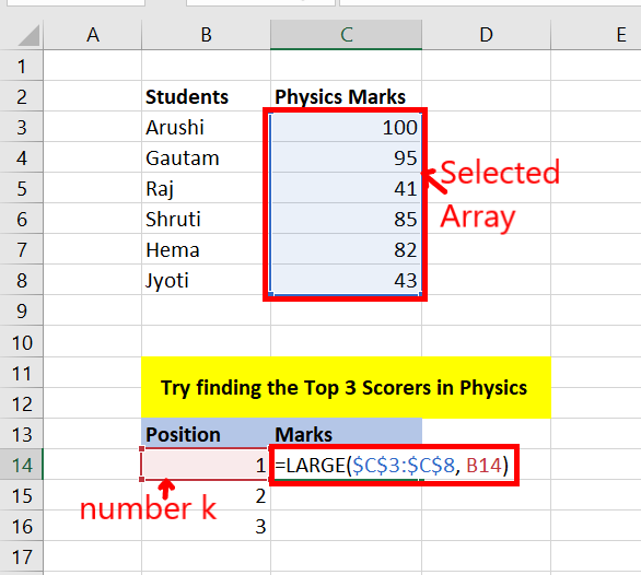
Steps for finding Top N values

Step 1: Use = LARGE(Array, k) function to have kth largest number in an array. Press Enter. 

where,

• Array: It is the first argument of the LARGE function. We need to provide an absolute reference for this array.
• k: It is the second argument of the LARGE function. It specifies which largest number you want. We will provide a relative reference to this number.

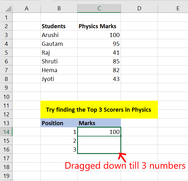
Step 2: You will get the kth largest number from the array. Now, drag down till the N numbers you want. For example: drag down to 3 cells for the given data set. 

Step 3: You have obtained the highest 3 marks scored by students. 

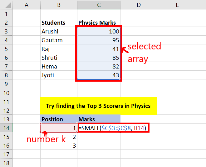
How to Find Bottom N values in Excel

Consider the same data set of Students and their Marks. Try finding the lowest 3 marks obtained by students. 

Steps for finding Bottom N values

Step 1: Use = SMALL(Array, k) function to have k^th smallest number in an array. For example, if the value of k is 1, then the function will return the smallest number in the array. If the value of k is 2, then the function will return the second smallest number in the array. Press Enter.

where, 

• Array: It is the first argument of the SMALL function. We need to provide an absolute reference for this array.
• k:  It is the second argument of the SMALL function. It specifies which smallest number you want. We will provide a relative reference to this number.

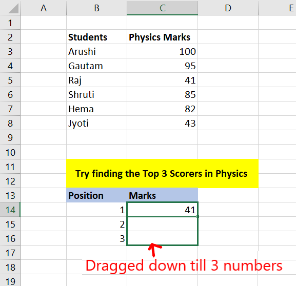
Step 2: You will get the kth smallest number from that array. Now, drag down till the N numbers you want. For example: drag down to 3 cells for the given data set. 

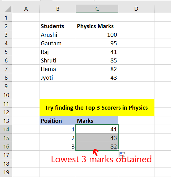
Step 3: You have obtained the lowest 3 marks scored by students. 

Additional Tips for Using LARGE and SMALL Functions

• Combining with Other Functions: You can combine LARGE and SMALL with other functions like IF to add more complex conditions.
• Dynamic Arrays: Use dynamic array formulas for larger datasets to make your calculations more efficient.
• Sorting Data: While LARGE and SMALL functions help find specific values, sorting your data can also give you a quick overview of the highest and lowest values.

Conclusion

In conclusion, understanding and using the LARGE and SMALL functions in Excel can significantly enhance your data analysis capabilities. By mastering cell references and knowing how to apply these functions, you can efficiently find the top and bottom N values in any dataset in Excel.

How to find Top or Bottom N values in Excel? – FAQs

How do I find the top N values in Excel?

To find the top N values in Excel, use the LARGE function. For example, =LARGE(A1:A10, 1) finds the highest value, =LARGE(A1:A10, 2) finds the second highest value, and so on. Drag the formula down to get the top N values.

How can I find the bottom N values in Excel?

To find the bottom N values in Excel, use the SMALL function. For example, =SMALL(A1:A10, 1) finds the smallest value, =SMALL(A1:A10, 2) finds the second smallest value, and so on. Drag the formula down to get the bottom N values.

What is the formula to find the Nth largest value in Excel?

The formula to find the Nth largest value in Excel is =LARGE(array, k), where array is the range of cells you are evaluating, and k is the position of the value you want.

How do I find the Nth smallest value in Excel?

Use the formula =SMALL(array, k) to find the Nth smallest value in Excel, where array is the range of cells, and k is the position of the value you want.

Can I use cell references with the LARGE and SMALL functions?

Yes, you can use cell references with the LARGE and SMALL functions. For example, =LARGE($A$1:$A$10, B1) uses the value in cell B1 to determine which largest number to find in the range A1 to A10.

How do I use the LARGE function to find multiple top values in Excel?

To find multiple top values, use the LARGE function with relative references for k. For example, =LARGE($A$1:$A$10, ROW(A1)) and drag the formula down to find the top values in the range.

How do I dynamically find the top or bottom N values in a dataset?

To dynamically find the top or bottom N values, use dynamic array formulas or helper columns that adjust the range or criteria based on your input.

What is the difference between the LARGE and SMALL functions in Excel?

The LARGE function returns the Nth largest value in a dataset, while the SMALL function returns the Nth smallest value. Both functions require an array and a position (k) as arguments.