How to Split Cells in Excel – Quick Steps

• Open MS Excel
• Select Data
• Go to the Data tab.
• Click Text to Columns.
• Choose Delimited and click Next

Splitting cells in Excel is a powerful technique that allows you to organize and manipulate your data with precision. If you’re dealing with names, addresses, or any other type of information stored in a single cell, learning how to split cells in Excel can significantly enhance your data management capabilities. This process involves splitting Excel cells into multiple cells, making it easier to analyze and work with specific data points.

By learning how to split cell in Excel, you can ensure your spreadsheets are not only more organized but also more efficient, allowing for quicker data analysis and reporting. Get ready to streamline your workflow and take your Excel skills to the next level with this essential guide on how to split cells in Excel.

How to Spilt Cells in Excel

What are Split Cells in Excel

Splitting cells in Excel is essential for dividing data within a single cell into separate cells. Splitting a cell in excel allows you to extract and organize information in a structured way, which makes it easier to analyze and present the data.

Most often, we need to excel cell split for text processing [E.g. Split Last Name and First Name from Customer name field].  

In the below data set, Column A has both Products and categories combined with a space delimiter.

Dataset

How to Split Cells Using Text to Columns Wizard in Excel

Step 1: Select the Data

Select the entire data set [Range A1 – A11].

Step 2: Go to the Data Tab

Go to “Data” >> Click “Text to Columns”, to pop up Convert Text to Columns Wizard.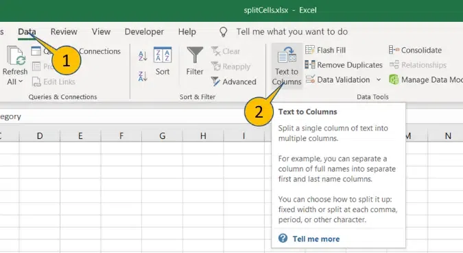

Go to Data Tab >> Click on “Text to Columns”

Step 3: Select “Delimited” and Press “Next”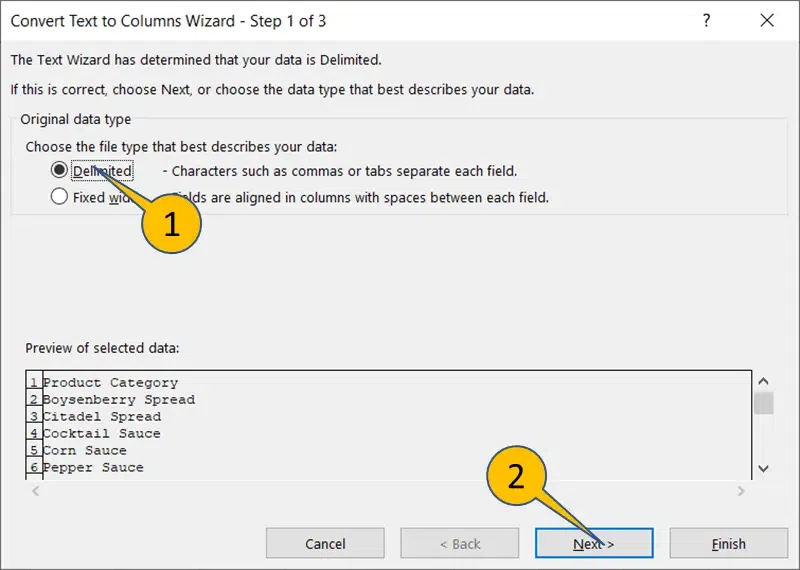

Select “Delimited” >> Press “Next”

Step 4: Check “Space” and Press “Next”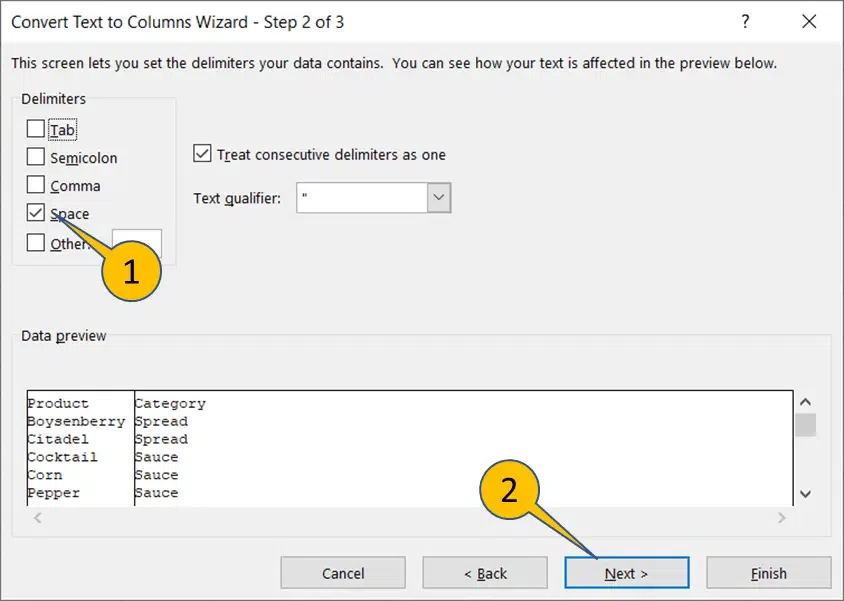

Check Space >> Press Next

Step 5: Change Destination to $B$1 cell and Press “Finish”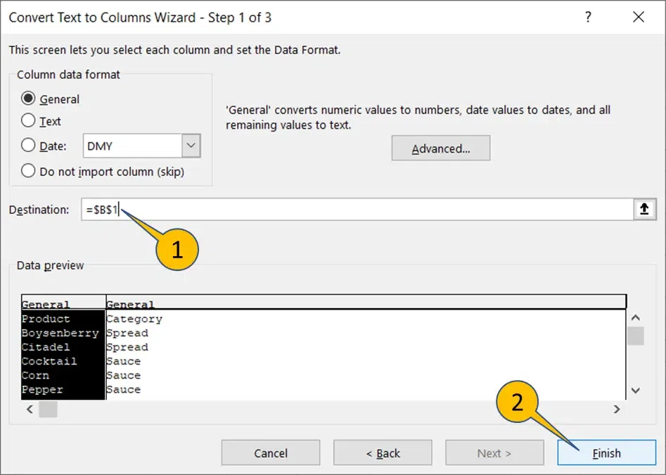

Enter Destination >> Click “Ok”

Step 6: Cells Splitted

Split Cells Achieved

How to Split Cells Using Excel Formulas in Excel

Step 1: Type Headers

Type Header text “Product” and “Category” to cells B1 and C1 respectively

Step 2: Enter Formula

Write the below formula in cell B2 to split the first word (Product)

=LEFT(A2,FIND(” “,A2)-1)

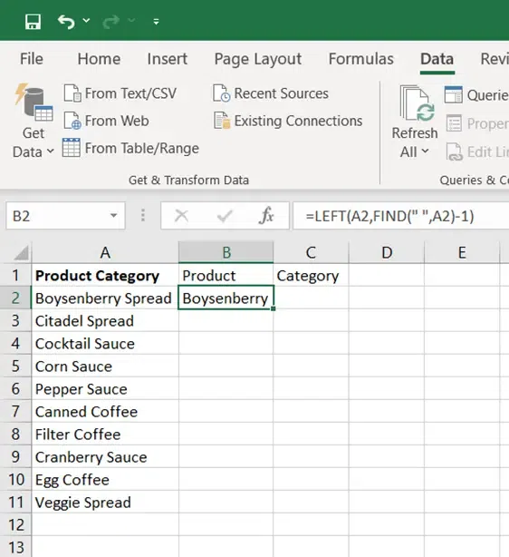Type Header

Step 3: Fill the formula in cells B2:B11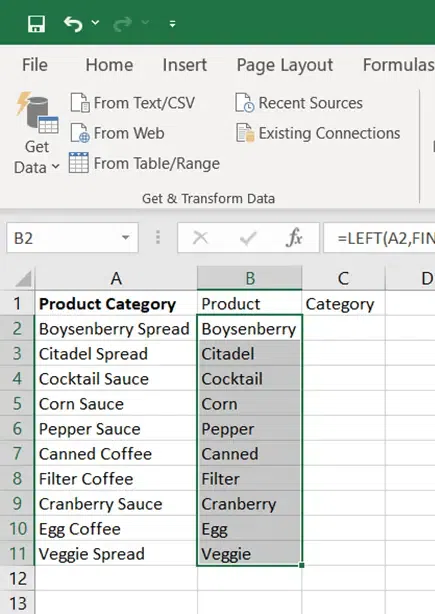 

Enter Formula

Step 4: Enter Formula in C2

Write the below formula in cell C2 to split the last word (Category)

=RIGHT(A2,LEN(A2)-FIND(” “,A2))

Write Formula in C2

Step 5: Fill the formula in cells C2:C11

Fill the Formula from C2:C11

How to Split Cells Using Flash Fill in Excel

Excel cell splitting using basic patterns is fairly simple to utilize. It can run in two possible ways:

• In the background
• Triggered manually by the user

Background execution

In this, Excel automatically offers ideas after trying to identify trends in the text.

Step 1: Type the Text Element

Type the text element we want to extract in the first row of the first column (with the source cells on the left). Enter the portion of the text from the second cell that we wish to extract. Flash Fill now takes action and offers suggestions.

Type the text

Step 2: Press Tab Key

To accept the suggested fill, press the Tab or Enter key.

Enter Key

Manual Execution

Now that we’ve seen how the Flash fill auto-suggests the data, let’s have a look at the manual approach as well.

Manual Execution

Step 1: Type the Text Element

In any single row, type the text element that has to be extracted. In this particular example (Last name)

Step 2: Go to the Home Tab

Click Home Tab and  Fill (dropdown) > Flash Fill, and choose the cells in the range that should have values entered.

Go to the Home Tab >> Click on “Fill Tab”

How to Split Cells Using Power Query in Excel

Excel’s Power Query feature can also be used to divide several cells. It has been natively available since Excel 2016.

Let’s start off with adding our data cells into the Power Query editor. The steps to take are listed below,

Step 1: Go to the Home Tab

Click Data tab and from Table/Range after choosing any cell from the data set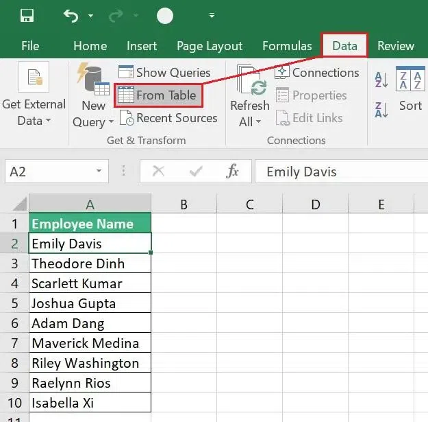

Go to the Data Tab

Step 2. Click “Ok”

Make sure the “My table has headers” option is checked, and the whole range is selected. Then press OK.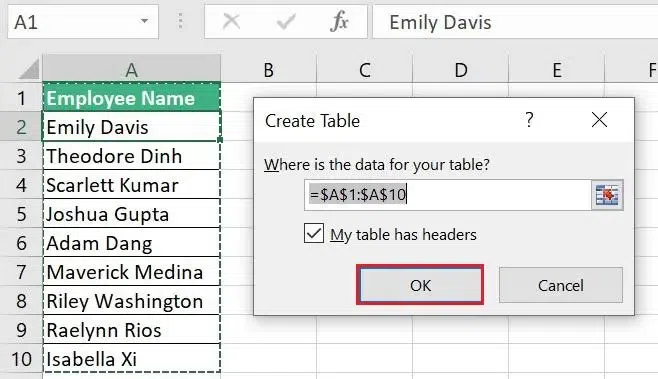

Click “Ok”

Step 3. Data Visible

All the data will be visible when the Power Query editor opens.

Step 4. Go to the Home Tab

Select Home > Split Column (drop-down) > By Delimiter from the Power Query ribbon.

Go to the Home Tab

Step 5. Click “Ok”

The Space character and At each occurrence of the delimiter are both suitable choices for our circumstances. Select OK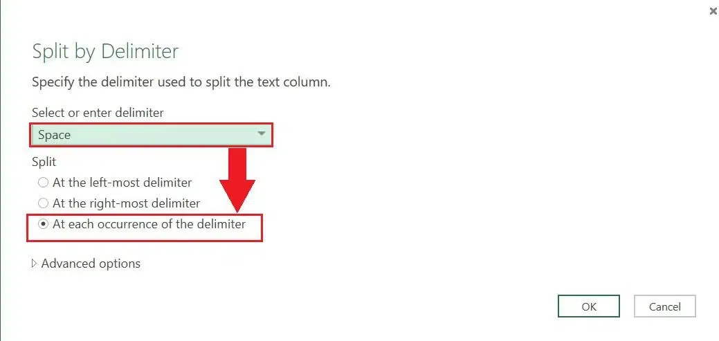

Select “Ok”

Step 6. Change Heading If necessary

The Employee name column is now divided into two distinct columns in the data preview pane. To change the headings to First name and Last name, double-click the header and make changes respectively.

Double Click the header to change

How to Split Cells in Excel Using Text Functions in Excel

There are many Text Functions in Excel, but we don’t need all of them here. A few of them are mentioned below:

• LEN- Returns the length of a String.
• RIGHT– Extract a specified number of characters from a String’s right end.
• LEFT- Extract a specified number of characters from a String’s left end.
• FIND– Look for a string inside another string.
• SEARCH– Return the positions of a string inside another string.
• MID– Extract a specified number of characters from a String’s center.

You can use any combination of the above text Functions to achieve your excel splitting cells.

Enter the Formula =LEFT(A2,SEARCH(” “,A2)-1) in cell B2.

The SEARCH looks for any space in the customer name and returns its position in the string. Then, the LEFT function extracts the part of the String from the left side, up to the position returned by the SEARCH Function. Now you are done with excel split cell.

Also Read:

• What is a Cell in Excel
• Excel: Modifying Columns, Rows, and Cells

Conclusion

In summary, learning cell splitting in excel is a valuable skill that can greatly improve your data management and presentation. If you need to separate names, addresses, or other combined data, knowing how to split a cell in Excel allows for more organized and readable spreadsheets. The techniques discussed, from using the Text to Columns feature to employing formulas, provide you with versatile options to handle various data scenarios. By implementing these methods of split cells in Excel, you’ll enhance your efficiency and accuracy in managing data, making your tasks easier and your results more professional.

How to Split Cells in Excel – FAQs

How do I split a single cell into multiple columns in Excel?

To split a single cell into multiple columns in Excel, use the “Text to Columns” feature. Select the cell or range of cells, go to the “Data” tab, click on “Text to Columns,” choose the delimiter or fixed width option, and follow the prompts to split the content into multiple columns.

What is the shortcut for split cells in Excel?

Excel does not have a direct keyboard shortcut for splitting cells. However, you can access the “Text to Columns” feature using Alt + A + E.

How to split cells in Excel vertically?

To split cells in Excel vertically, you can use the “Text to Columns” feature. Select the cell or range of cells, go to the “Data” tab, click on “Text to Columns,” choose the delimiter or fixed width option, and follow the prompts to split the content into multiple columns vertically.

How do I split cell size in Excel?

To split cell size in Excel, you can merge and unmerge cells to adjust the layout. Select the cells you want to merge or unmerge, right-click, and choose “Merge & Center” to combine cells or “Unmerge Cells” to split them back into individual cells. Alternatively, you can adjust the row height and column width to customize the cell size.

How to split a cell horizontally in excel?

Follow the steps given below:

1. Select the cells
2. Go to the “Data” tab
3. Choose “Fixed Width”
4. Specify where you want to break your cell
5. Pick a format option