NumPy is a fundamental package for scientific computing in Python, providing support for arrays, mathematical functions, and more. One of its powerful features is the ability to perform polynomial fitting using the polyfit function. This article delves into the technical aspects of numpy.polyfit, explaining its usage, parameters, and practical applications.

What is Polynomial Fitting?

Polynomial fitting is a form of regression analysis where the relationship between the independent variable xand the dependent variable y is modeled as an n-degree polynomial. The goal is to find the polynomial coefficients that minimize the difference between the observed data points and the values predicted by the polynomial.

Syntax and Parameters:

The numpy.polyfit function fits a polynomial of a specified degree to a set of data using the least squares method. The basic syntax is:

numpy.polyfit(x, y, deg, rcond=None, full=False, w=None, cov=False)

• x: array_like, shape (M,): x-coordinates of the M sample points (x[i], y[i]).
• y: array_like, shape (M,) or (M, K): y-coordinates of the sample points. Multiple datasets with the same x-coordinates can be fitted at once by passing a 2D array.
• deg: int: Degree of the fitting polynomial.
• rcond: float, optional: Relative condition number of the fit. Default is len(x) * eps, where eps is the machine precision.
• full: bool, optional: If True, return additional diagnostic information.
• w: array_like, shape (M,), optional: Weights to apply to the y-coordinates.
• cov: bool or str, optional: If True, return the covariance matrix of the polynomial coefficient estimates.

NumPy’s polyfit Function : Practical Examples

Let’s explore how to use numpy.polyfit with a practical example.

1. Linear Fit

A linear fit is a first-degree polynomial fit. Consider the following data points:

import numpy as np
import matplotlib.pyplot as plt

x = np.array([0, 1, 2, 3, 4, 5])
y = np.array([0, 0.8, 0.9, 0.1, -0.8, -1.0])

# Perform linear fit
coefficients = np.polyfit(x, y, 1)
print("Linear Fit Coefficients:", coefficients)

# Create polynomial function
p = np.poly1d(coefficients)

plt.scatter(x, y, label='Data Points')
plt.plot(x, p(x), label='Linear Fit', color='red')
plt.legend()
plt.show()

Output:

Linear Fit Coefficients: [-0.30285714  0.75714286]

Linear Fit

2. Higher-Degree Polynomial Fit

For higher-degree polynomials, the process is similar. Here is an example with a cubic polynomial:

# Perform cubic fit
coefficients = np.polyfit(x, y, 3)
print("Cubic Fit Coefficients:", coefficients)

# Create polynomial function
p = np.poly1d(coefficients)

# Plot data and fit
xp = np.linspace(-1, 6, 100)
plt.scatter(x, y, label='Data Points')
plt.plot(xp, p(xp), label='Cubic Fit', color='green')
plt.legend()
plt.show()

Output:

Cubic Fit Coefficients: [ 0.08703704 -0.81349206  1.69312169 -0.03968254]

Higher-Degree Polynomial Fit

Handling Multiple Datasets

numpy.polyfit can handle multiple datasets with the same x-coordinates by passing a 2D array for y. This is useful for fitting multiple curves simultaneously.

import numpy as np
import matplotlib.pyplot as plt

x = np.array([0, 1, 2, 3, 4, 5])
y_multi = np.array([[0, 0.8, 0.9, 0.1, -0.8, -1.0], [0, 0.7, 0.85, 0.05, -0.75, -0.95]])

# Perform linear fit on each dataset separately
coefficients_multi = [np.polyfit(x, y, 1) for y in y_multi]
print("Linear Fit Coefficients for Multiple Datasets:", coefficients_multi)

xp = np.linspace(-1, 6, 100)
plt.scatter(x, y_multi[0], label='Dataset 1')
plt.scatter(x, y_multi[1], label='Dataset 2')
for coeff in coefficients_multi:
    p = np.poly1d(coeff)
    plt.plot(xp, p(xp), label=f'Fit: {coeff}')
plt.legend()
plt.show()

Output:

Linear Fit Coefficients for Multiple Datasets: [array([-0.30285714,  0.75714286]), array([-0.28285714,  0.69047619])]

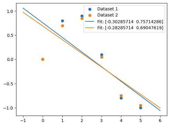
Handling Multiple Datasets

Advanced Options With NumPy’s polyfit Function

1. Weights

Weights can be applied to the y-coordinates to give different importance to different data points.

# Weights
weights = np.array([1, 1, 1, 1, 1, 10])

# Perform weighted fit
coefficients_weighted = np.polyfit(x, y, 1, w=weights)
print("Weighted Fit Coefficients:", coefficients_weighted)

Output:

Weighted Fit Coefficients: [-0.36783784  0.84378378]

2. Covariance Matrix

The covariance matrix of the polynomial coefficient estimates can be returned by setting cov=True.

# Perform fit with covariance
coefficients, cov_matrix = np.polyfit(x, y, 1, cov=True)
print("Fit Coefficients:", coefficients)
print("Covariance Matrix:", cov_matrix)

Output:

Fit Coefficients: [-0.30285714  0.75714286]
Covariance Matrix: [[ 0.0213551  -0.05338776]
 [-0.05338776  0.1957551 ]]

Conclusion

NumPy’s polyfit function is a versatile tool for polynomial fitting, offering various options to customize the fitting process. Whether you are performing a simple linear fit or a complex multi-dataset fit, numpy.polyfit provides the functionality needed to accurately model your data. With the introduction of the new polynomial API, working with polynomials in NumPy has become even more efficient and user-friendly.