|
|
In this article, we will learn about Contractive Autoencoders which come in very handy while extracting features from the images, and how normal autoencoders have been improved to create Contractive Autoencoders. What is Contarctive AutoEncoder?Contractive Autoencoder was proposed by researchers at the University of Toronto in 2011 in the paper Contractive auto-encoders: Explicit invariance during feature extraction. The idea behind that is to make the autoencoders robust to small changes in the training dataset. To deal with the above challenge that is posed by basic autoencoders, the authors proposed adding another penalty term to the loss function of autoencoders. We will discuss this loss function in detail. Loss Function of Contactive AutoEncoderContractive autoencoder adds an extra term in the loss function of autoencoder, it is given as: [Tex]\lVert J_h(X) \rVert_F^2 = \sum_{ij} \left( \frac{\partial h_j(X)}{\partial X_i} \right)^2[/Tex] i.e. the above penalty term is the Frobenius Norm of the encoder, the Frobenius norm is just a generalization of the Euclidean norm. In the above penalty term, we first need to calculate the Jacobian matrix of the hidden layer, calculating a Jacobian of the hidden layer with respect to input is similar to gradient calculation. Let’s first calculate the Jacobian of the hidden layer: [Tex]\begin{aligned}Z_j &= W_i X_i \\ h_j &= \phi(Z_j)\end{aligned}[/Tex] where \phi is non-linearity. Now, to get the jth hidden unit, we need to get the dot product of the ith feature vector and the corresponding weight. For this, we need to apply the chain rule.
[Tex]\begin{aligned} \frac{\partial h_j}{\partial X_i} &= \frac{\partial \phi(Z_j)}{\partial X_i} \\ &= \frac{\partial \phi(W_i X_i)}{\partial W_i X_i} \frac{\partial W_i X_i}{\partial X_i} \\ &= [\phi(W_i X_i)(1 – \phi(W_i X_i))] \, W_{i} \\ &= [h_j(1 – h_j)] \, W_i \end{aligned}[/Tex] The above method is similar to how we calculate the gradient descent, but there is one major difference, that is we take h(X) as a vector-valued function, each as a separate output. Intuitively, For example, we have 64 hidden units, then we have 64 function outputs, and so we will have a gradient vector for each of that 64 hidden units. Let diag(x) be the diagonal matrix, the matrix from the above derivative is as follows: [Tex]\frac{\partial h}{\partial X} = diag[h(1 – h)] \, W^T[/Tex] Now, we place the diag(x) equation to the above equation and simplify: [Tex]\begin{aligned}\lVert J_h(X) \rVert_F^2 &= \sum_{ij} \left( \frac{\partial h_j}{\partial X_i} \right)^2 \\[10pt] &= \sum_i \sum_j [h_j(1 – h_j)]^2 (W_{ji}^T)^2 \\[10pt] &= \sum_j [h_j(1 – h_j)]^2 \sum_i (W_{ji}^T)^2 \\[10pt]\end{aligned}[/Tex] Relationship with Sparse AutoencoderIn sparse autoencoder, our goal is to have the majority of components of representation close to 0, for this to happen, they must be lying in the left saturated part of the sigmoid function, where their corresponding sigmoid value is close to 0 with a very small first derivative, which in turn leads to the very small entries in the Jacobian matrix. This leads to highly contractive mapping in the sparse autoencoder, even though this is not the goal in sparse Autoencoder. Relationship with Denoising AutoencoderThe idea behind denoising autoencoder is just to increase the robustness of the encoder to the small changes in the training data which is quite similar to the motivation of Contractive Autoencoder. However, there is some difference:
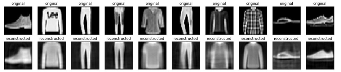
Contractive Autoencoder (CAE) Implementation StepwiseImport the TensorFlow and load the datasetBuild the Contractive Autoencoder (CAE) ModelDefine the loss functionDefine the GradientTrain the modelOutput: Epoch: 0 Generate resultsOutput:
|
Reffered: https://www.geeksforgeeks.org
| Machine Learning |

Type: | Geek |
Category: | Coding |
Sub Category: | Tutorial |
Uploaded by: | Admin |
Views: | 12 |